A Valuation-Aware, Scenario-Based Capital Markets Outlook

Implications for Portfolio Construction, Retirement Income, Sequence-of-Returns Risk,
and the AI Infrastructure Boom Using a Forward-Looking 10-Year Time Horizon

August 17, 2026

by Chris Brown, Ph.D., CFP^® and Ron A. Rhoades, JD, CFP^®

Client Consultation Notice

We invite clients and friends to schedule a consultation with Ron and Chris to discuss how the market developments and valuation dynamics described below may impact your personal retirement, asset allocation, and wealth preservation plan. Please contact Cathy Rhoades to schedule a Zoom meeting or phone call.

Executive Summary

This report provides a comprehensive August 2026 update to our previous capital markets outlooks, incorporating valuation data, economic indicators, forward return expectations through August 14, 2026, and an in-depth examination of the artificial intelligence (AI) capital expenditure boom (Rhoades & Brown, 2025, 2026; Cahn, 2024). Over the past six months, global equity markets have extended a remarkable multi-year bull run, characterized in mid-2026 by significant broadening into small-capitalization stocks, international developed equities, and emerging markets, alongside continued momentum in technology and AI-driven growth sectors (Vanguard Group, 2026a; Research Affiliates, 2026). However, beneath this strong price momentum, fundamental valuation metrics for U.S. large-company stocks have reached historical extremes, driven in large part by immense corporate spending on AI infrastructure (Campbell & Shiller, 1988; Shiller, 2015; Goldman Sachs Research, 2024). Starting valuations dictate long-term expected returns, and current entry prices severely compress forward return potential while magnifying sequence-of-returns risk for retirees (Pfau & Kitces, 2014).

A note on how to read this report. Much of what follows is technical, and it is written for clients and fellow professionals alike. Wherever a specialized term appears for the first time we define it in ordinary language, and each major section closes with a short plain-English summary. Readers who want the conclusions without the evidence should read the five plain-English takeaways at the end of this Executive Summary, then Part X on whether an expensive market justifies a more conservative allocation, and then the practical guidance in Part XI.

As fiduciary advisers, our mandate requires looking past short-term market enthusiasm to analyze the mathematical framework that governs long-term wealth accumulation and distribution. Our primary findings include:

S. Large-Cap Equities Remain Stretched Near Historic Valuation Peaks. The S&P 500 Shiller Cyclically Adjusted Price-to-Earnings (CAPE) ratio stood at 42.56 as of August 14, 2026 (Multpl, 2026a). Across 1,866 monthly observations since 1871, only ten readings have exceeded this level, and every one of them fell between April 1999 and August 2000, surrounding the December 1999 all-time peak of 44.19 (Shiller, 2015; Multpl, 2026a). Corroborating measures – including a trailing twelve-month price-to-earnings ratio of 30.00 against a long-run mean of 16.23, and a Price-to-Book ratio of 6.18x against a long-run mean of 3.16x – confirm that U.S. mega-cap stocks trade at profound premiums to historical fundamentals. (Multpl, 2026b, 2026c) The price-to-book figure cited here is drawn from the single-vendor Multpl series; the multi-vendor dataset underlying Tables 1B, 1C, and 3 reports 5.26x for the S&P 500, and the source note to Table 1B explains why differing aggregation conventions produce the gap.
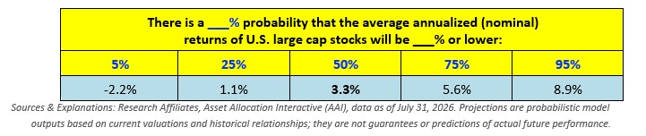
Forward 10-Year Return Expectations are Heavily Muted for U.S. Large-Caps. Latest simulations from the Vanguard Capital Markets Model® (VCMM) as of June 30 / July 22, 2026 project 10-year nominal average annualized U.S. equity returns of 4.2% to 6.2%, down from a range of 4.9% to 6.9% three months earlier as valuations stretched further, while Research Affiliates Asset Allocation Interactive (AAI) forecasts a 10-year nominal expected average annualized return of just 3.3% for U.S. large-cap stocks. (Vanguard Group, 2026a; Research Affiliates, 2026)
A better way of viewing expected returns is through the lens of probabilities:

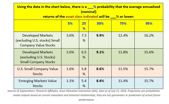
Superior Expected Returns Reside in Non-U.S. Value and Small-Cap Segments. Because non-U.S. and small-cap value asset classes trade at substantial valuation discounts relative to U.S. mega-caps, forward return models project compelling risk premiums. For instance, Research Affiliates projects 10-year nominal average annualized returns of 9.9% for Developed ex-U.S. Small Cap Value, 9.1% for Developed ex-U.S. Small Cap, 8.6% for U.S. Small Cap Value, and 8.4% for Emerging Markets Value. (Research Affiliates, 2026; Vanguard Group, 2026a)

Eleven Alternative Valuation Yardsticks Mostly Agree – and the Exceptions Are Instructive. Because no single ratio is definitive, Part II of this report examines eleven alternative methods of valuing the stock market alongside the CAPE ratio. The Buffett Indicator – total U.S. stock market value divided by gross domestic product – stood at 218.1% for the first quarter of 2026, roughly 56.6% above its long-term trendline and the fourth-highest reading ever recorded (Nash, 2026; Current Market Valuation, 2026). Robert Shiller’s Excess CAPE Yield, which measures the extra return stocks offer over Treasury bonds, fell to 0.92 as of August 1, 2026, against a long-run average of 2.52 (GuruFocus, 2026). By contrast, the S. stock market’s forward price-to-earnings ratio of 20.0 as of August 7, 2026 sits only marginally above its five-year average of 19.9 (Butters, 2026). The gap between those readings is itself among the most important facts in this report, and Part II explains it.
Independent Research Organizations Have Reached Substantially the Same Conclusion. Vanguard’s assessment of conditions at June 30, 2026 places broad U.S. equity valuations at effectively the highest percentile it has ever observed (Vanguard Group, 2026b). AQR estimates a 3.9% annualized real return for U.S. large-cap stocks over the medium term, against 4.9% for developed markets outside the United States and 5.1% for emerging markets (AQR Capital Management, 2025). Cambridge Associates measures U.S. equities at 2.2 times the cyclically adjusted price-to-cash-earnings multiple of the rest of the world, roughly 50% above the long-run median relationship (Cambridge Associates, 2025). In contrast, J.P. Morgan projects 6.7% annualized for U.S. large-cap equities over 10 to 15 years, against 7.8% for emerging markets (J.P. Morgan Asset Management, October 2025). And in August 2026 emerging market stocks traded at 9.9 times forward earnings against more than 20 times for the S&P 500 – the first time in at least two decades that the emerging market multiple has been less than half the U.S. multiple (Bloomberg News, 2026).
AI Infrastructure Spending Faces a Multi-Trillion-Dollar Revenue Gap and Contagion Risks. Combined capital expenditures by the major U.S. hyperscalers reached approximately $410 billion in 2025, and consensus 2026 forecasts now cluster near $794 billion (Goldman Sachs Research, 2026). Bain & Company estimates the industry will require roughly $2 trillion in annual new revenue by 2030 to fund this buildout, and projects an $800 billion shortfall even under favorable adoption assumptions (Bain & Company, 2025; Cahn, 2024). Financial engineering (off-balance-sheet SPVs and 5–6 year depreciation stretching), low-cost Chinese open-weight models (DeepSeek), and free local desktop AI tools (like Bionic) threaten model pricing power. Insolvency in major pure-play AI labs could trigger cascading defaults across cloud vendors, semiconductor suppliers, private debt, and utility infrastructure. (Goldman Sachs Research, 2024; Barclays, 2024)
At Least One Sophisticated Institutional Investor Maintains Significant Dry Powder. Reflecting high valuation levels and scarce margin of safety, Berkshire Hathaway held $365.5 billion in cash and short-term Treasury bills at June 30, 2026 (28.9% of total assets), down from a record $397.4 billion (31.7%) at March 31, 2026 as incoming chief executive Greg Abel began deploying capital. Chairman Warren Buffett has long maintained that patience is essential when market prices leave little cushion for error. Berkshire’s cash position is evidence about Berkshire’s own opportunity set and risk tolerance, not a directive about what any individual retiree should hold. (Berkshire Hathaway, 2026; The Motley Fool, 2026)
- However, record dollar balances are not the same as ample cushion. Bank of America’s Global Fund Manager Survey for July 2026 recorded average cash allocations among surveyed managers of 3.6%, down from 4.1% a month earlier and low enough to trigger that survey’s contrarian sell signal (Bank of America Global Research, 2026). Retail money market fund assets stood at a record $3.10 trillion for the week ended August 12, 2026, within a $7.93 trillion total (Investment Company Institute, 2026). Measured against an equity market capitalization that has risen faster still, however, the proportional cushion available to absorb a shock is thinner than the dollar figures suggest.
Sequence-of-Returns Risk is Elevated for Near-Term and Recent Retirees. When retirement withdrawals commence during an extreme valuation regime, early market drawdowns cause permanent capital impairment (Pfau & Kitces, 2014). To counteract this risk, we advocate three core structural guardrails: rising equity glidepaths with a bond tent, dynamic/valuation-aware withdrawal rules, and multi-factor asset class diversification. (Pfau & Kitces, 2014; Guyton & Klinger, 2006; Fama & French, 2018)
Growing More Conservative Because the Market Is Expensive Requires Two Correct Decisions, Not One. Part X examines the academic literature on tactical asset allocation and market timing. Valuation-based switching rules have not survived honest out-of-sample testing (Fisher & Statman, 2006; Goyal & Welch, 2008), and of 34 tactical allocation funds identified in 2013, only 12 survived the following decade – not one of which beat a plain 60/40 portfolio (Ptak, 2023). The deeper difficulty is structural: a tactical shift is not complete until the portfolio is restored, so the investor must be right about when to leave and right about when to return, and Blanchett estimates that a tactical strategy must be correct roughly 70% of the time after taxes merely to match a static allocation (Sharpe, 1975; Blanchett, 2011). We therefore reallocate within equities on valuation grounds rather than reducing equity exposure on a forecast, and treat an actual reduction as warranted only when a client’s plan, stage of life, or true risk tolerance calls for it (Kitces & Pfau, 2015).

This Report in Plain English: Five Takeaways for Clients

Clients who do not work in finance may find the following summary sufficient. Everything that follows in Parts I through XI is the supporting evidence.

Stocks are expensive, and expensive is not the same as doomed. Paying a high price for a stream of future profits does not cause a crash. What it reliably does is lower the return you earn over the following decade, because you have paid more for each dollar of earnings you will eventually receive (Campbell & Shiller, 1988; Shiller, 2015). Nothing in this report predicts when, or whether, prices will fall.
Most of the expense sits in large U.S. growth companies. U.S. large-cap growth stocks trade at 11.50 times book value. U.S. small-cap value stocks trade at 1.72 times, and international developed small-cap value at 1.42 times. Diversifying away from the most expensive corner of the market does not require predicting anything; it requires only continuing to own what is cheap alongside what is dear (Fama & French, 2018; Research Affiliates, 2026).
The forecasts in this report are ranges, not predictions. When Research Affiliates projects 3.3% a year for U.S. large-cap stocks, the honest reading is that a decade of anywhere from roughly –2.2% to +8.9% a year is consistent with their model (Research Affiliates, 2026). A plan built on a single number is fragile. A plan built to survive the range is not.
If you are within roughly ten years of retirement, the order of your returns matters more than their average. A portfolio that averages 6% but loses money in years one through three can fail where an identical portfolio, earning the same average in a different order, succeeds (Pfau & Kitces, 2014). Parts VI, VII, and IX describe the three structural defenses we use against this risk.
Nothing here calls for dramatic action. The appropriate response to high valuations is not to leave the market. It is to rebalance systematically, to hold meaningful weightings outside U.S. mega-cap growth, and – if you are retired or nearly so – to hold enough short- and intermediate-term fixed income that you never have to sell stocks at a bad price to pay for groceries (Kitces, 2014; Benz, 2024).

Click here to download our Capital Markets Outlook.

Part I: The Mid-2026 Market Advance and Updated Valuation Backdrop

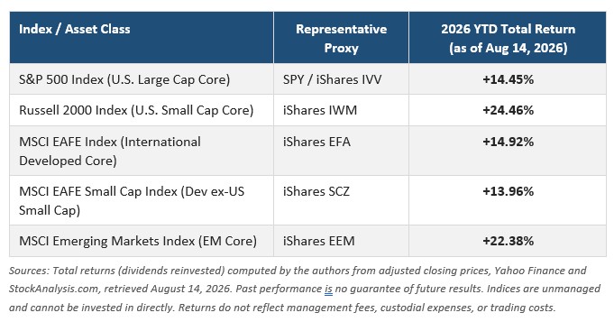
The first seven months of 2026 extended the robust equity advance that generated three consecutive years of double-digit U.S. equity total returns through 2025 (+26.3% in 2023, +25.0% in 2024, and +17.9% in 2025) (Towfighi, 2025). A defining characteristic of the 2026 advance has been market rotation and style broadening. While 2023–2025 performance was heavily dominated by a small cohort of U.S. mega-cap technology firms (the ‘Magnificent Seven’), 2026 year-to-date performance exhibits powerful outperformance in smaller-capitalization stocks, international developed markets, and emerging markets (Vanguard Group, 2026a).

A Plain-English Guide to the Terms Used in This Report

The tables and analysis that follow rely on a small number of technical terms. Each is defined here once, in ordinary language, and then used consistently throughout.

Price-to-Earnings (P/E) ratio. The price of a share divided by the company’s annual profit per share. A P/E of 20 means investors are paying $20 for each $1 of annual profit. A higher number means a more expensive stock.
Shiller CAPE ratio. The same idea, except that the denominator is the average of the past ten years of inflation-adjusted profits rather than a single year. Averaging ten years removes the distortion caused by recessions and booms. Robert Shiller, awarded the Nobel Prize in Economics in 2013, demonstrated that this measure bears a meaningful relationship to the returns investors earn over the following decade (Campbell & Shiller, 1988; Shiller, 2015).
Price-to-Book (P/B) ratio. The market price of a company divided by its accounting net worth – assets minus liabilities. A P/B of 5 means investors are paying five dollars for each dollar of net assets carried on the balance sheet. This measure has become less reliable for technology companies, whose most valuable assets – software, brands, accumulated research – frequently do not appear on the balance sheet at all.
Percentile rank. Where today’s reading falls among all past readings. A 99.6th percentile reading means the measure was lower than it is now in 99.6% of the months examined, and higher in only 0.4%.
Z-score, or standard deviations from the mean. A measure of how unusual a reading is. Roughly two-thirds of historical readings fall within one standard deviation of the average, and about 95% fall within two. A reading of +2.32 standard deviations therefore lies outside the range that contains 95% of recorded history.
Nominal versus real return. A nominal return is the raw percentage gain. A real return subtracts inflation and describes what the money will actually buy. Unless stated otherwise, the return forecasts in this report are nominal.
Sequence-of-returns risk. The risk that a poor run of markets arrives early in retirement, while withdrawals are being taken. Two retirees can earn identical average returns across thirty years and finish with very different outcomes depending on the order in which those returns arrived (Pfau & Kitces, 2014).

Valuations Remain Near Historic Extremes for U.S. Large Company Stocks

While near-term market momentum remains robust, starting valuations govern long-term return potential (Campbell & Shiller, 1988; Shiller, 2015). A rigorous evaluation of core U.S. large-cap valuation metrics reveals an exceptionally stretched environment:

Shiller CAPE Ratio (42.56 as of August 14, 2026): The S&P 500 Shiller CAPE ratio sits at 42.56, approximately 2.6 times its 155-year historical median of 16.11 and well above its long-run mean of 17.40 (Multpl, 2026a). Across 1,866 monthly observations beginning in February 1871, only ten readings have exceeded this level – all of them between April 1999 and August 2000, surrounding the December 1999 all-time peak of 44.19 – and the current reading stands well above the September 1929 pre-Depression peak of 32.56 and the November 2021 pre-bear-market peak of 38.58. (Multpl, 2026a; Shiller, 2015)
Trailing Price-to-Earnings Ratio (30.00 as of August 14, 2026): The S&P 500’s price-to-earnings ratio, computed on trailing twelve-month as-reported earnings, stood at 30.00, against a long-run mean of 16.23 and a median of 15.08 measured since 1917 (Multpl, 2026b). Investors are paying roughly 1.8 times the historical norm for each dollar of realized corporate profit. Unlike the CAPE ratio, this measure draws on only the most recent year of earnings, and it therefore flatters the market whenever profit margins are unusually high – as they are today.
Price-to-Book Ratio (6.18x): The aggregate S&P 500 P/B ratio stands at 6.18x, vastly exceeding the 3.16x mean and 2.91x median of the 105 quarter-end observations reported since December 1999 (Multpl, 2026c). Current market prices trade at an extraordinary premium to the underlying corporate net asset value. (Multpl, 2026c)
One Measure Disagrees, and the Disagreement Is Informative: The market’s forward price-to-earnings ratio – price divided by the earnings Wall Street analysts expect over the coming twelve months – stood at 20.0 as of August 7, 2026, only marginally above its five-year average of 19.9 and its ten-year average of 19.0 (Butters, 2026). Read in isolation, that measure would describe an ordinary market. It reaches that conclusion because it accepts the analyst consensus at face value, and in mid-2026 that consensus embeds both record profit margins and continued rapid earnings growth. We examine this divergence, together with ten other valuation frameworks, in Part II.

U.S. large company stocks, as represented by the S&P 500® Index, account for approximately 80% of available (float-adjusted) U.S. equity market capitalization (S&P Dow Jones Indices, 2026). However, there are many ways to ‘slice and dice’ the stock market, and many other asset classes that can be created – and then examined. In the pages that follow we examine various asset classes, applying the Fama-French factors to specify the asset classes we examine.

Selection Rationale: Why the 2003–2026 Baseline Period (23.6 Years)?

To establish a rigorous, unbiased empirical framework for evaluating current valuation metrics, we selected January 1, 2003 as the baseline starting date for our multi-asset historical analysis. Selecting January 2003 provides a clean, post-bubble baseline where valuations were grounded and not artificially stretched:

Valuation Neutrality Post-Tech Bubble Collapse: The early 2000s marked the resolution of the late-1990s technology bubble. Following the 2000–2002 bear market reset, equity price-to-earnings and price-to-book ratios returned to reasonable historical norms (S&P 500 price-to-book fell from a peak of 5.06x at March 31, 2000 to a trough of 2.43x at September 30, 2002, and stood at 2.58x at March 31, 2003). Starting in 2003 avoids anchoring historical averages to extreme dot-com bubble distortions while providing a healthy, non-stretched baseline. (Shiller, 2015; Multpl, 2026c)
Coverage of Four Complete Macroeconomic & Market Cycles: The 23.6-year window from January 2003 through August 2026 incorporates four full market cycles: (a) the 2003–2007 post-tech recovery and credit expansion; (b) the 2007–2009 Global Financial Crisis (GFC) and severe debt de-leveraging; (c) the 2009–2020 zero-interest-rate policy (ZIRP) and Quantitative Easing (QE) expansion; and (d) the post-2020 COVID shock, subsequent 2022–2023 rate-tightening regime, and the 2023–2026 artificial intelligence expansion. (Vanguard Group, 2025, 2026a)
Data Consistency Across Multiple Global Asset Classes: By utilizing a continuous monthly dataset spanning 284 months (January 2003 to August 2026), we ensure data alignment across all different global style factors and international regions – including specialized small-cap value and emerging market sub-indices. (Research Affiliates, 2026)

Table 1B: Price-to-Book Values: Current vs. 23.6-Year Historical Valuation Summary Table (2003–2026)

Table 1B presents current August 2026 Price-to-Book (P/B) ratios alongside 23.6-year historical averages, medians, percentile ranks, and standard deviations from the mean (Z-scores) across all 19 global asset classes. Ratios in Tables 1B and 1C are drawn from the authors’ multi-vendor dataset and are stated as of August 1, 2026. Because index providers, fund sponsors, and data vendors differ in how they aggregate book value – weighted harmonic mean versus aggregate sum, and differing treatment of negative book values – these figures will not always tie precisely to the single-source Multpl series cited in Part I, nor to the current characteristics published on individual index and fund fact sheets. Readers comparing across sources should confirm the convention and the as-of date before drawing conclusions from small differences.

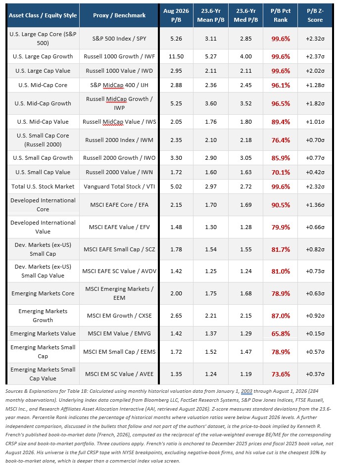
Profound Valuation Overextension in U.S. Large Growth and Total Market: U.S. Large Cap Core (S&P 500) and Total U.S. Stock Market trade at P/B ratios of 5.26x and 5.02x, placing them in the 99.6th percentile of historical observations over the past 23.6 years (+2.32σ above their long-term means). U.S. Large Cap Growth exhibits even more severe multiple expansion, trading at 11.50x P/B (+2.37σ). Over 284 months of historical data, current U.S. mega-cap growth valuations have virtually no precedent outside the final months of major market speculative tops. (See Table 1B and its accompanying source note.)

Implications for Strategic Allocation: While the “dot-com bubble” of 1999-2000 saw extreme overvaluations in U.S. growth stocks, and only modest overvaluations for small cap and value stocks, in August 2026 the U.S. large-cap, total-market and growth asset classes are significantly overvalued, and some are extremely so. The evidence is more mixed for value and small-cap value, where our data and the academic series cited below disagree. (Vanguard Group, 2026a; Fama & French, 2018)

An Independent Check, and Where It Diverges: Kenneth French’s published book-to-market data corroborates this report’s central claim about U.S. large growth: his implied price-to-book for large-cap growth is 11.00x against the 11.50x shown above, at the 95th percentile and +2.09σ of its own 2003–2026 range. His broad large-cap and total-market figures (4.65x and 4.35x) are likewise consistent in direction.

The value segments, however, diverge. On French’s data U.S. small-cap value sits at the 17.7th percentile of its own range and −0.76σ, and U.S. large-cap value at the 41st percentile and −0.15σ – that is, at or below their long-term norms rather than above them. Measured from December 2002 to December 2025, his large growth portfolio re-rated by 107% and small growth by 60%, while large value rose 4% and small value fell 1%. Part of the gap is definitional, since French’s value cut is deeper than a commercial index screen, but the direction of travel is unambiguous and it argues that the re-rating of the past two decades is concentrated in growth rather than distributed across every asset class. (French, 2026)

A re-rating refers to a long-term structural shift where the market permanently assigns higher valuation multiples, such as Price-to-Earnings or Price-to-Book ratios, to specific assets. Over the past two decades, this upward valuation adjustment has not occurred uniformly across the entire economy. Instead, the re-rating has been heavily concentrated within high-innovation growth stocks, particularly technology companies. This uneven expansion has widened the valuation gap between asset-light growth firms and traditional, asset-heavy value sectors.

For a client, the practical question is whether that re-rating is permanent. If it is, today’s prices are defensible and the forward returns in Table 3 are too pessimistic. If it reverses, those forward returns are the ones that matter.

Table 1C: Historical Price-to-Book (P/B) Across Major Market Cycles (2003–2026)

To illustrate how asset class valuations have evolved across economic expansions, liquidity crises, and market cycles, Table 1C tracks Price-to-Book (P/B) multiples across eight key market cycle inflection points between January 2003 and August 2026.

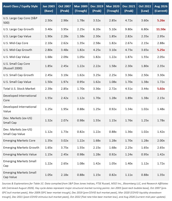
Unprecedented Expansion in U.S. Large Growth vs. Pre-GFC and Post-COVID Peaks: During the pre-Great Financial Crisis (pre-GFC) market peak in October 2007, U.S. Large Cap Core traded at a P/B of 2.98x and U.S. Large Growth traded at 3.95x. In December 2021, driven by zero interest rates and massive fiscal stimulus, Large Growth peaked at 9.80x P/B. As of August 2026, U.S. Large Growth has expanded further to an extraordinary 11.50x P/B – nearly triple its 2007 pre-crisis peak level. (See Table 1C and its accompanying source note.)

Is Book Value Still Relevant? With the continued rise of the technology sector, and the increase in intangible property held by corporations (which is not always reflected in book values), the use of the price-book ratio has come under scrutiny. Software code, patent portfolios, brand value, and accumulated research are among a modern corporation’s most valuable assets, yet accounting rules generally require that the spending which created them be expensed rather than capitalized, so they never appear as book value at all.

The massive increase in the price-to-book ratio for the U.S. Large Growth stock asset class is directly driven by the rise of technology firms, which structurally carry far less physical book value on their balance sheets. Standard accounting rules treat corporate spending on software, data networks, and research as immediate expenses rather than capitalized assets. Consequently, these modern giants command massive market valuations while their official book values remain artificially low. This fundamental mismatch inflates historical valuation metrics, suggesting that traditional book value has largely become of lesser value for measuring modern corporate wealth.

A 60-year analysis of U.S. stocks covering 1963 through 2022 concluded that price-to-book remains “a superior choice for practical investment solutions” among competing value metrics (Ahn & Saito, 2023). On balance, we treat price-to-book as most informative for value and small-cap segments, where tangible assets dominate enterprise value, and least informative for U.S. large-cap growth, which is why Part II’s eleven additional valuation measures carry the greater weight for that segment of the market.

Given the conflicting opinions on the use of price-to-book ratios for valuation purposes, we do not rest our conclusions on the price-to-book ratio alone. Part II examines eleven additional valuation frameworks, several of which do not depend on book value in any way.

Independent Corroboration: What Leading Research Organizations Concluded in Mid-2026

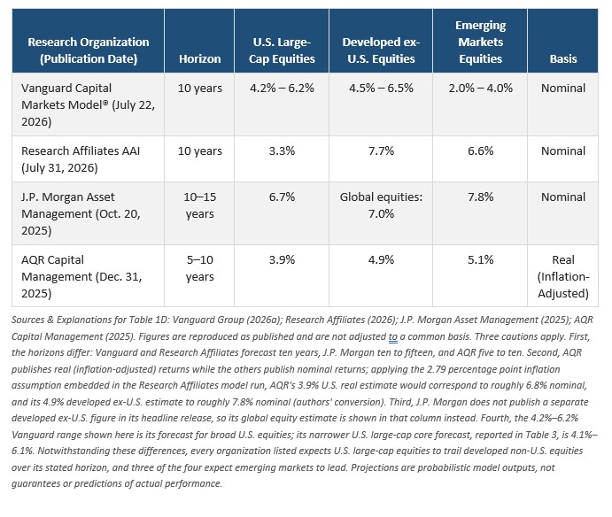
A valuation analysis that cites only itself is of limited use to a client. Between October 2025 and August 2026, most of the major research organizations that publish long-horizon return estimates reached conclusions consistent with those set out above, using different data, different models, and different definitions of value. We summarize their published positions here and reproduce their headline numbers in Table 1D.

In its assessment of market conditions as of June 30, 2026, Vanguard described broad U.S. equity valuations as reaching effectively the highest percentile it has ever observed, up from the 99.7th percentile three months earlier. Within the U.S. market, Vanguard found that growth stocks moved from the 58th to the 77th percentile of their fair-value range during the second quarter, that small-capitalization stocks became materially more expensive, and that value stocks alone remained closer to fair value than either (Vanguard Group, 2026b). Vanguard pairs this with an explicit caution that valuations are poor predictors of short- and intermediate-term performance and should not by themselves drive allocation changes (Vanguard Group, 2026a, 2026b).
Writing on July 9, 2026, Morningstar’s chief U.S. market strategist reported that Morningstar’s equity analysts had raised fair value estimates on several mega-capitalization stocks in response to substantial realized earnings growth, pushing market prices close to those revised estimates, and that what discount remained in the market was concentrated in artificial-intelligence mega-caps rather than distributed broadly (Sekera, 2026). Morningstar’s bottom-up method – building a discounted cash flow valuation company by company – is methodologically independent of every ratio discussed above, which is precisely why its more benign conclusion deserves attention.
P. Morgan Asset Management. J.P. Morgan’s 2026 Long-Term Capital Market Assumptions, the thirtieth annual edition, project 6.7% annualized returns for U.S. large-cap equities over a 10-to-15-year horizon, 7.0% for global equities, and 7.8% for emerging market equities, with a traditional 60/40 portfolio at 6.4%. J.P. Morgan attributes the emerging market advantage to more attractive cyclical starting points and expected currency appreciation (J.P. Morgan Asset Management, 2025).
AQR Capital Management. AQR’s 2026 capital market assumptions estimate medium-horizon real (inflation-adjusted) returns of 3.9% for U.S. large-cap equities, 4.9% for developed markets outside the United States, and 5.1% for emerging markets, against 2.4% for ten-year U.S. Treasuries. AQR observes that the U.S. CAPE ratio of nearly 40 sits at the 96th percentile of readings since 1980, and that the growth advantage markets are pricing into U.S. equities exceeds AQR’s own forecast – which is why the United States carries the lowest expected return among major developed markets in their framework (AQR Capital Management, 2025).
Cambridge Associates. Cambridge Associates measures valuation using cyclically adjusted price-to-cash-earnings, a variant that substitutes cash earnings for accounting earnings. On that basis the MSCI US Index traded at 2.2 times the multiple of the MSCI ACWI ex-US Index, approximately 50% above the long-run median relationship, and still 25% above it after neutralizing differences in sector composition. Cambridge Associates recommends a modest overweight to non-U.S. equities and an overweight to developed market small-capitalization equities (Cambridge Associates, 2025).
Dimensional Fund Advisors. Dimensional reports that the ten largest stocks in the S&P 500 represented over 40% of the index at year-end 2025, roughly double their weight a decade earlier, and observes that in 2025 the MSCI World ex USA and MSCI Emerging Markets indices each returned over 30% against 17% for the Russell 3000 – a reminder that the global diversification which felt costly for a decade began to pay in 2025 (Dimensional Fund Advisors, 2026).
Research Affiliates. Research Affiliates’ Asset Allocation Interactive model, the source of the forecasts in Tables 3 and 3B below, projects a 3.3% nominal ten-year return for U.S. large-cap stocks against 9.9% for developed ex-U.S. small-cap value, on data as of July 31, 2026 (Research Affiliates, 2026).
Market pricing itself. On August 10, 2026, the MSCI Emerging Markets Index traded at 9.9 times forward earnings against more than 20 times for the S&P 500 – the first time in at least two decades that the emerging market multiple has been below half the U.S. multiple (Bloomberg News, 2026). Separately, the MSCI EAFE Value Index returned 33.8% in 2025, its strongest calendar year in more than twenty-five years, and at October 31, 2025 EAFE value stocks still traded at nearly twice the earnings yield of EAFE growth stocks (Gupta, 2025).

Table 1D: Published Long-Horizon Equity Return Estimates From Major Research Organizations

Table 1D collects the headline equity return estimates published by four organizations that disclose long-horizon forecasts by region. The figures are reproduced exactly as each organization published them, which means they are not directly comparable; the source note explains the three differences that matter.

Part II: Beyond a Single Ratio – Eleven Alternative Ways to Measure Whether the Stock Market Is Expensive

Every valuation ratio is an argument about what a share of stock is worth, and every one of them is incomplete. The Shiller CAPE ratio relied upon in Part I compares price to a ten-year average of past earnings. That choice makes the measure stable, but it also makes it slow to recognize genuine and durable improvements in corporate profitability. Critics have argued for years that the CAPE overstates how expensive the market is, and some of those criticisms are well founded (Masturzo & Kunz, 2017; White & Haghani, 2024).

A fiduciary analysis should therefore not rest on any single measure. In this Part we set out eleven alternative frameworks that professional investors use to judge whether stocks are expensive. For each we explain the idea in ordinary language, report the most recent published reading, and state plainly what the measure does and does not tell us. Readers will notice that the eleven do not agree with one another. The pattern of that disagreement – which measures conclude ‘ordinary’ and which conclude ‘extreme’ – turns out to be more informative than any single number, and we reconcile it at the end of this Part.

Group One: Measures Anchored to Current or Expected Earnings

Trailing price-to-earnings ratio. Price divided by the past twelve months of actual reported profits. It is the simplest measure available and requires no forecast of any kind. As of August 14, 2026 the S&P 500’s trailing ratio stood at 30.00, against a mean of 16.23 and a median of 15.08 measured since 1917 (Multpl, 2026b). Its weakness is that a single year of profits can be unusually good or unusually bad, and a measure that calls stocks cheap in the middle of a profit boom is not much help. Signal: expensive, at roughly 1.8 times the historical norm.
Forward price-to-earnings ratio. Price divided by the profits Wall Street analysts expect over the coming twelve months. As of August 7, 2026 this stood at 20.0, against a five-year average of 19.9 and a ten-year average of 19.0 (Butters, 2026). This is the most benign of the twelve measures examined in this report, and its benignity is instructive: the measure is benign only because it accepts the analyst consensus. Analyst estimates have historically been optimistic over long horizons, and in mid-2026 they embed both record profit margins and rapid artificial-intelligence-driven earnings growth. Signal: modestly expensive – conditional on those forecasts proving correct.
The Rule of 20. A rule of thumb holding that the sum of the market’s price-to-earnings ratio and the rate of inflation should equal roughly 20 at fair value. The logic is that inflation erodes the real value of future earnings, so a higher inflation rate justifies a lower multiple (Charles Schwab, 2026). U.S. consumer prices rose 3.4% over the twelve months ended July 2026 (U.S. Bureau of Labor Statistics, 2026). Adding that to the forward multiple of 20.0 produces 23.4, about 17% above the rule’s fair-value threshold; adding it to the trailing multiple of 30.00 produces 33.4, roughly 67% above (authors’ computation from Butters, 2026; Multpl, 2026b; U.S. Bureau of Labor Statistics, 2026). The rule was devised roughly three decades ago, when profit margins, index sector composition, and monetary policy all differed considerably from today. Signal: expensive on either input.

Group Two: Measures Anchored to Long-Run Average Earnings

The payout-adjusted CAPE (P-CAPE). The most serious academic criticism of the Shiller CAPE, and the one clients most deserve to understand, is that the ratio has drifted upward over time for a mechanical reason unrelated to speculation. James White and Victor Haghani demonstrated that because companies now retain and reinvest a far larger share of their profits than they once did – the dividend payout ratio averaged 65% from 1880 to 1988, fell to 45% from 1988 to 2024, and has recently run near 35% – a simple ten-year average of past earnings systematically understates the earnings power those retained profits have since built. Adjusting for this, their payout-adjusted cyclically adjusted earnings figure averaged 19% higher than the traditional measure across 1890 to 2024, and their payout-adjusted earnings yield explained 35% of the variation in subsequent ten-year real returns, against 24% for the traditional version (White & Haghani, 2024). Signal: expensive, but meaningfully less extreme than a raw CAPE of 42.56 implies. This is the strongest technical argument against the most alarming reading of Part I, and we state it here in full rather than bury it.
Cyclically adjusted price-to-cash-earnings (CAPCE). A variant that substitutes cash earnings for accounting earnings, on the view that cash is harder to reshape through accounting choices – including, notably, the depreciation-schedule extensions discussed in Part III of this report. Cambridge Associates reports that on this basis the MSCI US Index traded at 2.2 times the multiple of the MSCI ACWI ex-US Index, roughly 50% above the long-run median relationship between them, and remained 25% above the median even after neutralizing differences in sector composition (Cambridge Associates, 2025). Signal: U.S. equities expensive relative to the rest of the world – and not merely because the United States is home to more technology companies.

Group Three: Measures That Compare Stocks to Bonds

The Fed Model and the implied equity risk premium. The Fed Model compares the market’s earnings yield – profits divided by price, the inverse of the P/E ratio – to the yield on the ten-year Treasury note. If bonds yield more than stocks earn, bonds look relatively attractive. Schwab reported this comparison in negative territory as of late November 2025 (Charles Schwab, 2026). A more rigorous version is Aswath Damodaran’s implied equity risk premium, which solves for the return investors must be expecting given today’s prices and today’s cash flow forecasts, then subtracts the risk-free rate. Damodaran computed an implied premium of 4.23% entering 2026, against a ten-year Treasury yield of 3.97% in late February 2026, rising to a range of 4.37% to 4.51% during the March 2026 oil and Middle East disruption (Damodaran, 2026). Signal: mixed. The premium is thin but not negative, so stocks are not being priced as though equity risk were free. The Fed Model’s weakness is that earnings are not delivered to shareholders the way bond coupons are, and the comparison ignores both inflation and future growth.
Shiller’s Excess CAPE Yield (ECY). Shiller’s own answer to the objection that the CAPE ratio ignores interest rates. The ECY takes the inverse of the CAPE ratio – the cyclically adjusted earnings yield – and subtracts the real ten-year Treasury yield, producing an estimate of the extra return stocks offer over bonds. As of August 1, 2026 the ECY stood at 0.92, against a long-run average of 2.52 and a median of 3.3, and roughly 39% below its level a year earlier (GuruFocus, 2026). Signal: expensive. This matters because crediting stocks for low interest rates is the single most common defense of current prices – and even after doing so, the compensation for owning equities instead of Treasuries is well under half its historical norm.

Group Four: Measures That Compare Stocks to the Real Economy or to Assets

The Buffett Indicator. Total U.S. stock market capitalization divided by gross domestic product, a measure Warren Buffett once described as probably the best single indicator of where valuations stand at any given moment (Buffett & Loomis, 2001). Jennifer Nash reported the ratio at 218.1% for the first quarter of 2026 – 56.6% above its long-term trendline, or 1.8 standard deviations, and the fourth-highest reading in the history of the series (Nash, 2026). A parallel calculation put the ratio at 219% as of March 31, 2026, approximately 2.1 standard deviations above trend, reflecting $69.15 trillion of market value against $31.57 trillion of annualized gross domestic product (Current Market Valuation, 2026). Signal: strongly expensive. Two well-founded objections apply: U.S.-listed companies earn a substantial share of their profits abroad, which inflates the numerator without affecting the domestic denominator, and the measure ignores interest rates entirely.
Tobin’s Q. Developed by Nobel laureate James Tobin, this measure divides the market value of corporate assets by what it would cost to replace them. The economic logic is compelling: if a company’s shares are worth far more than the cost of rebuilding the company from scratch, either the shares are overpriced or competitors will build a rival and compete the premium away. Its practical weakness in 2026 is severe. The replacement cost of a semiconductor fabrication plant can be estimated; the replacement cost of a trained large language model, a patent portfolio, or a global brand cannot, and high inflation further distorts replacement cost calculations (Charles Schwab, 2026). Signal: directionally expensive, but we place limited weight on any precise reading, for the same reason we caution against over-reliance on the price-to-book ratio.
Market capitalization to corporate gross value added. A refinement of the Buffett Indicator that replaces economy-wide gross domestic product with the value added by non-financial corporations specifically, thereby removing government, housing, and financial sector output from the denominator and correcting part of the mismatch. John Hussman, who has advanced this measure for many years, described conditions in June 2026 as the most extreme point in U.S. stock market history, and no less extreme than the 1929 and 2000 bubble peaks, observing that the S&P 500 information technology sector traded at 45 times earnings on a record 30% operating profit margin – more than three times its historical norm (Hussman, 2026). Signal: extremely expensive. Readers should weigh this alongside the fact that the same analyst has maintained a bearish posture for an extended period, and that a measure which has signaled extreme overvaluation for years has been of no use whatever for timing.

Group Five: Measures Built From the Bottom Up

Bottom-up intrinsic valuation. Rather than applying any ratio to the index as a whole, this approach values each company individually by discounting its projected future cash flows back to a present value, then aggregates the results. Morningstar maintains such estimates across its analyst coverage universe; in July 2026 its chief U.S. market strategist reported that analysts had raised fair value estimates on several mega-capitalization companies on the strength of realized earnings growth, leaving market prices close to those revised estimates, with the residual discount concentrated in artificial-intelligence mega-caps (Sekera, 2026). Aswath Damodaran applies the same discounted cash flow logic at the index level (Damodaran, 2026). Signal: roughly fair. This is the second of the twelve measures to reach a benign conclusion, and it does so for a closely related reason – it is anchored to forecasts of the future rather than to the historical record.

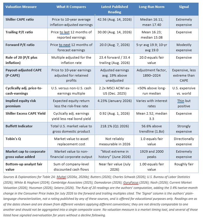
Table 2A: What Twelve Valuation Measures Say About U.S. Stocks in Mid-2026

Table 2A places the Shiller CAPE ratio discussed in Part I alongside the eleven alternative measures described above, so that readers can see the full weight of evidence in one view.

Reconciling the Disagreement: Why Two Honest Measures Give Opposite Answers

Nine of the twelve measures in Table 2A describe a market that is expensive to extremely expensive. Two – the forward price-to-earnings ratio and bottom-up analyst fair value – describe a market that is close to ordinary, and one, the implied equity risk premium, sits between the two camps. Understanding why is far more useful to a client than memorizing any single figure.

The measures divide cleanly along one line. Those anchored to what corporations have actually earned in the past, or to the size of the economy that generates those earnings, conclude that the market is extremely expensive. Those anchored to what corporations are forecast to earn in the future conclude that the market is roughly normal. The entire gap between the two camps is an argument about the durability of profit margins.

Corporate profit margins in the United States are at or near record levels; the S&P 500 information technology sector alone carries an operating margin above 30%, more than three times its historical norm (Hussman, 2026). Forward-looking measures assume those margins persist. Backward-looking measures implicitly assume they revert toward historical averages, as margins have after every previous period of extraordinary profitability. Neither assumption is unreasonable on its face. But the two cannot both be correct, and a portfolio constructed as though the optimistic one were certain is not a fiduciary portfolio.

There is a second and narrower point on which we owe readers candor. The most credible technical criticism of the Shiller CAPE – that falling dividend payout ratios have mechanically inflated it – is correct, and it means the raw reading of 42.56 overstates the degree of overvaluation (White & Haghani, 2024). It does not, however, reverse the conclusion. The payout adjustment raises the earnings denominator by roughly 19% on average, which would bring an equivalent reading down materially but nowhere near historical norms; and the adjustment does not touch the Buffett Indicator, the Excess CAPE Yield, the price-to-book ratio, the Rule of 20, or the international comparison, each of which arrives at the same conclusion by an entirely independent route.

In plain English: the U.S. stock market is expensive on most measures, and roughly fair only on the two measures that assume today’s exceptional corporate profitability continues indefinitely. That is not, by itself, a reason to sell anything. It is a reason to be honest with yourself about what you are counting on, and to make certain that your retirement does not require the optimistic assumption to be correct.

Part III: The AI Infrastructure Boom – CapEx Realities, Off-Balance-Sheet Financing, Hardware Obsolescence, Open-Source Disruption, and Systemic Contagion Risks

A primary catalyst driving U.S. large-cap equity valuations to their current historic extremes has been the unprecedented surge in corporate capital expenditures (CapEx) dedicated to artificial intelligence infrastructure (Goldman Sachs Research, 2024; Cahn, 2024). Investors have enthusiastically bid up mega-cap technology firms and semiconductor manufacturers under the premise that AI represents a transformative general-purpose technology. However, as fiduciary advisers evaluating long-term risk and return, we must analyze whether the financial math underpinning this investment boom is economically sustainable – or whether the ecosystem is building a classic structural bubble vulnerable to a sharp correction (Barclays, 2024; Morgan Stanley, 2024).

The Unprecedented Scale of Capital Spending in Big Tech Today

The sheer volume of capital being committed to AI hardware and data centers by U.S. hyperscalers – principally Microsoft, Alphabet, Meta, and Amazon – alongside specialized venture-backed AI labs (such as OpenAI, Anthropic, and xAI) has reached historic proportions (Goldman Sachs Research, 2024; Morgan Stanley, 2024). Combined capital expenditures across these major technology platforms reached approximately $410 billion in 2025 across Microsoft, Alphabet, Meta, and Amazon, and 2026 forecasts now range from roughly $760 billion to $794 billion, with the higher consensus figure computed on a five-company basis that adds Oracle (Goldman Sachs Research, 2026; Statista, 2026).

To put this spending in perspective, modern AI CapEx is directed toward four core infrastructure pillars:

High-Performance Accelerator Silicon: Procurement of specialized Graphics Processing Units (GPUs) and Tensor Processing Units (TPUs) – such as NVIDIA’s H100, H200, Blackwell B200, and upcoming Rubin architectures, alongside custom ASICs like Google’s TPU v5/v6 and AWS Trainium. (Goldman Sachs Research, 2024)
Hyperscale Data Center Real Estate & Cooling: Construction of massive gigawatt-scale data center facilities equipped with specialized liquid-cooling infrastructure required to dissipate the extreme thermal output of dense GPU racks. (Barclays, 2024)
High-Speed Interconnect Networking: Deployment of high-bandwidth InfiniBand and ultra-high-speed Ethernet optical networking to connect tens of thousands of GPUs into unified training clusters. (Morgan Stanley, 2024)
Energy Infrastructure & Power Agreements: Direct investment in electrical substations, natural gas turbines, and long-term Power Purchase Agreements (PPAs) with nuclear and utility providers to secure massive base-load electricity supplies. (Goldman Sachs Research, 2024)

In plain English, current AI capital intensity rivals or exceeds the grandest infrastructure buildouts in economic history – including the 1840s British Railway Mania, the expansion of the U.S. electrical grid in the 1920s, and the fiber-optic telecom buildout of the late 1990s (Cahn, 2024). While historical infrastructure booms ultimately produced immense long-term social utility, they frequently resulted in severe short- to medium-term capital destruction for early equity investors who paid overinflated entry prices before actual commercial revenues materialized (Cahn, 2024; Shiller, 2015).

The Revenue Gap Math: Sequoia’s $600 Billion Question

The fundamental economic challenge confronting the AI ecosystem lies in the stark mismatch between capital spent and revenue generated (Cahn, 2024). In a widely cited economic analysis, David Cahn of Sequoia Capital framed this challenge in June 2024 as “AI’s $600 Billion Question” (Cahn, 2024). Cahn’s estimate rested on roughly $300 billion of annual AI data-center spending; because that figure has since more than doubled, the revenue gap he identified has widened materially.

The financial arithmetic governing hardware return on investment (ROI) is straight-forward:

Hardware & Total Cost Structure: For every $1 spent on specialized GPU silicon, an enterprise incurs approximately $1 in additional operational and capital expenses – including data center real estate, power, cooling, networking, and specialized machine learning engineering. (Cahn, 2024)
Revenue Requirement for Economic Profit: To cover hardware depreciation, operating expenses, energy costs, and deliver a reasonable return on invested capital (ROIC) to shareholders, current capital expenditure implies a need for roughly $2.5 trillion in annualized AI revenue (Galloway, 2026). Applying a documented bottom-up methodology, Bain & Company reaches a comparable conclusion, estimating a requirement of approximately $2 trillion in annual new revenue by 2030 and projecting an $800 billion shortfall even under favorable adoption assumptions (Bain & Company, 2025).
The Actual Revenue Reality: As of mid-2026, total estimated end-user AI revenue across the entire global economy – including enterprise copilot subscriptions, consumer ChatGPT/Claude premium accounts, and developer API token usage – is estimated at approximately $150 billion annually (Galloway, 2026). For context, Gartner separately estimates end-user spending on artificial intelligence models and platforms at $64.3 billion in 2026 (Gartner, 2026). On these figures, AI revenue would need to rise roughly seventeen-fold to justify the current level of capital expenditure.

This creates an extraordinary annual revenue gap (Cahn, 2024; Goldman Sachs Research, 2024). While supporters argue that enterprise software revenue will scale exponentially as AI models mature, adoption across broad enterprise workflows has progressed at a far more measured pace (Goldman Sachs Research, 2024). Companies face substantial integration hurdles, data security and privacy constraints, legal liability concerns, model ‘hallucination’ risks, and unclear productivity gains for routine administrative tasks (Goldman Sachs Research, 2024; Barclays, 2024). Unless end-user AI applications generate hundreds of billions in net new enterprise value, current capital spending levels will inevitably face a painful downward recalibration.

Off-Balance-Sheet Financing & Financial Engineering: Hiding the Leverage

To maintain high headline corporate earnings and protect traditional debt metrics, major technology firms and venture-backed AI providers are increasingly turning to financial engineering to fund data center expansion off their main corporate balance sheets (Barclays, 2024; Morgan Stanley, 2024).

Key off-balance-sheet mechanisms include:

Special Purpose Vehicles (SPVs) & Joint Ventures: Tech companies are forming joint ventures with private equity giants (e.g., Blackstone, Blue Owl, Apollo) and infrastructure funds to build data centers inside separate corporate entities. The tech giant agrees to lease the facility back upon completion, keeping the multi-billion-dollar construction debt off its balance sheet while recording only ongoing lease operating expenses. (Barclays, 2024)
GPU-Collateralized Private Debt Facilities: Emerging AI cloud providers (neo-cloud vendors) and specialized AI labs are pledging physical clusters of NVIDIA GPUs as loan collateral to secure billions in private credit. Private debt funds lend capital backed by the perceived secondary market value of the silicon chips. (Morgan Stanley, 2024)
Long-Term Take-or-Pay Power & Lease Liabilities: Hyperscalers are entering into decade-long, binding Sale-Leaseback agreements and power purchase contracts (PPAs) with utility providers. These structures create massive, un-cancellable future cash outflows that function economically like long-term corporate debt, even if they do not appear in traditional headline leverage ratios. (Barclays, 2024)

In plain English, off-balance-sheet financing masks the true financial leverage accumulated across the AI supply chain (Barclays, 2024). Just as off-balance-sheet vehicles masked leverage in the lead-up to the 2008 Global Financial Crisis and the late-1990s telecom crash, current structures obscure the total volume of debt dependent on unproven AI revenue streams (Barclays, 2024; Goldman Sachs Research, 2024).

Hardware Obsolescence and the Depreciation Schedule Illusion

A severe, underappreciated risk in data center accounting is the rapid pace of hardware obsolescence compared to official accounting depreciation schedules (Goldman Sachs Research, 2024; Morgan Stanley, 2024).

Over the past four years, major Big Tech firms adjusted their accounting policies by extending the useful life of server and network equipment from 3 years out to 5 or 6 years (Morgan Stanley, 2024). On paper, stretching depreciation schedules reduces annual depreciation expense, immediately boosting reported GAAP net income by tens of billions of dollars across the sector (Morgan Stanley, 2024).

However, this accounting treatment directly contradicts the economic reality of semiconductor innovation:

Accelerated Silicon Cycles: NVIDIA and competing chipmakers have compressed their product release cadence from a traditional 2-year cycle down to an aggressive 1-year cycle (Hopper in 2022/2023, Blackwell in 2024/2025, and Rubin in 2026). (Goldman Sachs Research, 2024)
Energy-Efficiency & Performance-per-Watt Disparities: Next-generation chips offer exponential improvements in energy efficiency (tokens generated per kilowatt-hour of electricity) and lower training/inference costs (Goldman Sachs Research, 2024). Because data center power and rack space are strictly constrained, operating an older GPU cluster (such as an A100 or H100) becomes economically unviable long before its physical hardware wears out. (Goldman Sachs Research, 2024; Barclays, 2024)
The Impairment Threat: Holding 5-to-6-year depreciation schedules for hardware that becomes economically obsolete in 2 to 3 years creates a growing accounting discrepancy. As newer, far more efficient chips flood the market, cloud operators will be forced to write down the value of legacy data centers, resulting in sudden, massive asset impairment charges that directly hit future corporate earnings. (Morgan Stanley, 2024; Goldman Sachs Research, 2024)

The Rise of Low-Cost Asian LLMs: Token Price Commoditization

While U.S. proprietary model developers (e.g., OpenAI, Anthropic, Google) have spent tens of billions of dollars training closed, ultra-large frontier models, global competition has emerged from China-based AI research institutions (e.g., DeepSeek, Qwen/Alibaba, Yi/01.AI, Moonshot) that are fundamentally disrupting the cost structure of artificial intelligence (DeepSeek-AI, 2024).

In late 2024 and early 2025, Chinese research lab DeepSeek released frontier open-weights models (DeepSeek-V3 and DeepSeek-R1) that matched or approached the performance of leading U.S. proprietary models on key benchmarks in coding, mathematics, and reasoning – at a tiny fraction of the training and operational cost (DeepSeek-AI, 2024; Guo et al., 2025). Kimi and Qwen models have followed.

Key technical breakthroughs enabling this low-cost disruption include:

Algorithmic Efficiency Innovations: Utilizing Multi-head Latent Attention (MLA), Mixture-of-Experts (MoE) architectures where only a fraction of total model parameters activate per token, and FP8 mixed-precision training techniques that reduce memory and compute requirements. (DeepSeek-AI, 2024)
Reinforcement Learning Optimization: Developing novel Group Relative Policy Optimization (GRPO) training methods that allow models to self-improve reasoning capabilities without requiring ultra-expensive human-labeled data sets. (Guo et al., 2025)
Token Price Collapse: Asian open-weight providers price flagship inference at roughly $0.14 to $0.44 per million input tokens and $0.28 to $0.87 per million output tokens, against roughly $1.00 to $5.00 input and $5.00 to $25.00 output for Western closed flagship models – a discount on the order of 80% to 95%. DeepSeek moved to peak and off-peak billing effective August 16, 2026, which raises its peak output rate to $1.32 to $3.96 per million tokens and narrows, but does not close, that gap. (DeepSeek, 2026; Barclays, 2024)

In plain English, the rapid emergence of high-quality, open-weight Chinese models commoditizes artificial intelligence (DeepSeek, 2026; Barclays, 2024). When high-capability inference tokens become cheap and freely available, closed-model vendors lose their pricing power and gross margin umbrellas (Barclays, 2024). This severely compresses the expected future software revenues needed to justify Western CapEx spending (Cahn, 2024; DeepSeek, 2026).

The Local Edge Revolution: Free, Downloadable Desktop AI

Compounding the commoditization of commercial cloud APIs is the rapid rise of downloadable, open-source AI applications designed to run locally on consumer and workstation hardware (Ollama, LM Studio, Jan, ExLlama).

For example, co-author Ron Rhoades recently downloaded ‘Bionic’ – a local, open-weights generative AI interface – directly onto his personal MacBook Pro. Operating entirely on local Apple Silicon hardware utilizing unified system memory, local desktop AI applications deliver compelling practical advantages over centralized cloud subscriptions:

Absolute Zero Operating Cost: Local desktop AI runs completely free of charge. Users incur no monthly software subscription fees ($20 to $30/month per user for ChatGPT Plus or Claude Pro) and zero per-token cloud API charges. (Barclays, 2024)
Uncompromising Data Security & Privacy: When utilizing local software like Bionic, personal files, financial spreadsheets, client data, and proprietary research remain strictly confined to the user’s local hard drive. Data is never uploaded over the internet, transmitted to external cloud servers, or exposed to third-party model training (which we have never done in the past, which has restricted our use of AI in certain analyses). (Barclays, 2024)
Low Latency & Offline Availability: Local execution provides instant response times without cloud server queue delays, internet bandwidth constraints, or external service outages. (Barclays, 2024)

For routine writing, editing, document summarization, coding assistance, and spreadsheet analysis, downloadable local models handle 80% to 90% of the daily tasks required by business professionals, educators, and researchers. By providing high-quality, secure AI functionality at zero marginal cost, edge-based local models threaten to cannibalize the consumer subscription and enterprise API revenue streams that centralized cloud providers rely upon to recoup their infrastructure investments (Cahn, 2024; Barclays, 2024).

Contagion Risk Analysis: What Happens If a Major AI Pure-Play Files Bankruptcy?

A central systemic question for investors is what happens if one or more leading venture-backed AI labs (e.g., pure-play providers like OpenAI, Anthropic, or similar entities) encounter a funding freeze – losing the ability to raise new equity rounds at elevated multi-billion-dollar valuations or secure debt – and are forced into restructuring or Chapter 11 bankruptcy (Goldman Sachs Research, 2024; Barclays, 2024).

Because the AI ecosystem is tightly interconnected through circular revenue contracts, equity-for-compute deals, and off-balance-sheet leases, the failure of a major AI provider would trigger a multi-stage financial contagion across several economic sectors:

Stage 1: Hyperscaler Cloud Revenue & Receivable Default: Leading AI labs maintain multi-billion-dollar long-term commitments to rent compute capacity from hyperscalers (g., Microsoft Azure, AWS, Google Cloud). An AI lab insolvency would immediately default on these cloud contracts, forcing hyperscalers to write off uncollected receivables and absorb sudden, massive excess data center capacity. (Goldman Sachs Research, 2024; Barclays, 2024)
Stage 2: Semiconductor & Supply Chain Order Cancellations: A cloud compute glut would cause hyperscalers to drastically cancel new hardware orders. Semiconductor designers (NVIDIA, AMD), foundry manufacturers (TSMC), memory producers (SK Hynix, Micron), and server OEMs (Dell, Supermicro) would experience a severe, unexpected order cliff, driving down semiconductor earnings and equity valuations across the tech supply chain. (Goldman Sachs Research, 2024; Morgan Stanley, 2024)
Stage 3: Private Debt & Data Center SPV Default Cascade: Specialized data center SPVs and neo-cloud providers that borrowed heavily against GPU collateral would face immediate loan defaults. Private credit funds, infrastructure funds, and syndicate banks holding GPU-backed debt would suffer credit losses and illiquidity, as the secondary market value of used GPUs collapses under forced liquidation. (Barclays, 2024; Morgan Stanley, 2024)
Stage 4: Energy & Utility Power Contract Stranding: Power companies and nuclear plant operators that signed binding PPAs and invested capital to build grid infrastructure for specific data centers would face defaulted contracts and stranded energy assets, impacting the utility sector. (Goldman Sachs Research, 2024)
Stage 5: Macro Equity Market Valuation Repricing: Because U.S. equity market indices are heavily concentrated in mega-cap technology firms (with the top 10 constituents accounting for approximately 37% of the S&P 500 as of August 14, 2026), an AI valuation unwind would drive a broad-based drawdown across the S&P 500 and Nasdaq 100, directly threatening retirees holding overweighted cap-weighted index portfolios. (Slickcharts, 2026; Shiller, 2015; Pfau & Kitces, 2014)

Some market observers and economists have opined in recent months that should such a bankruptcy filing occur, this could even launch the United States into a recession.

Fiduciary Summary & Strategic Investor Guidance

In summary, while artificial intelligence represents a genuine technological advancement, current stock market pricing reflects an extraordinary level of speculative optimism that ignores capital expenditure realities, off-balance-sheet leverage, rapid hardware obsolescence, low-cost Asian open-model competition, and edge-based local AI disruption (Cahn, 2024; Goldman Sachs Research, 2024; DeepSeek-AI, 2024).

For wealth managers and individual investors, these structural risks reinforce the imperative of disciplined fiduciary portfolio construction:

Avoid Cap-Weighted Mega-Cap Overconcentration: Recognize that traditional market-cap weighted U.S. indices (S&P 500) carry extreme concentration in richly valued technology firms exposed to AI CapEx risks. (Shiller, 2015; Fama & French, 2018)
Embrace Multi-Factor Diversification: Allocate capital across academically verified style factors – specifically U.S. Small Cap Value and Mid-Cap Value – which trade at grounded historical multiples and carry far less exposure to AI CapEx inflation. (Fama & French, 2018; Dimensional Fund Advisors, 2020)
Maintain International Value Exposure: Maintain meaningful weightings in Developed International Value and Emerging Markets Value equities, where forward expected returns are substantially higher and entry valuations provide a healthy margin of safety. (Research Affiliates, 2026; Vanguard Group, 2026a)
Protect Decumulation Portfolios with Structural Guardrails: For retirees, mitigate sequence-of-returns risk by utilizing a Rising Equity Glidepath paired with a Bond Tent and Three-Bucket framework to insulate living expenses from potential equity market repricing. (Pfau & Kitces, 2014; Benz, 2024)

Part IV: Scenario-Based Economic Framework

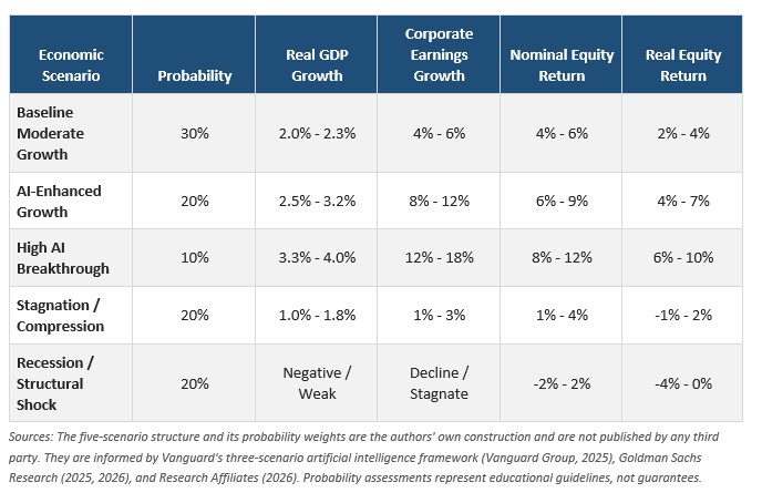
Given the inherent unpredictability of macroeconomic developments, prudent fiduciary planning requires probabilistic scenario modeling rather than relying on point forecasts (Ilmanen, 2011; Vanguard Group, 2025). We update our 10-year forward economic framework into five distinct scenarios, evaluating real GDP growth, corporate earnings, and expected equity returns under each backdrop:

Part V: Forward 10-Year Capital Market Assumptions Across 14 Equity Asset Classes and Three Fixed Income Benchmarks

To construct optimal portfolios and conduct robust retirement income stress testing, advisers must evaluate capital market assumptions across the full spectrum of global equity and fixed income asset classes (Masturzo & Kunz, 2017). Three U.S. mid-cap classes and two emerging-market small-cap classes are omitted from this section because neither Vanguard nor Research Affiliates forecasts them separately. Table 3 provides forward 10-year nominal return expectations sourced from the Vanguard Capital Markets Model® (simulations as of June 30, 2026) and Research Affiliates Asset Allocation Interactive (data as of July 31, 2026), covering 14 global equity asset classes alongside three fixed income benchmarks. Neither provider publishes a forecast for every one of these asset classes. Cells marked “Not published” indicate that the provider does not disclose an expected return at that level of granularity; no substitute estimate has been supplied in its place.

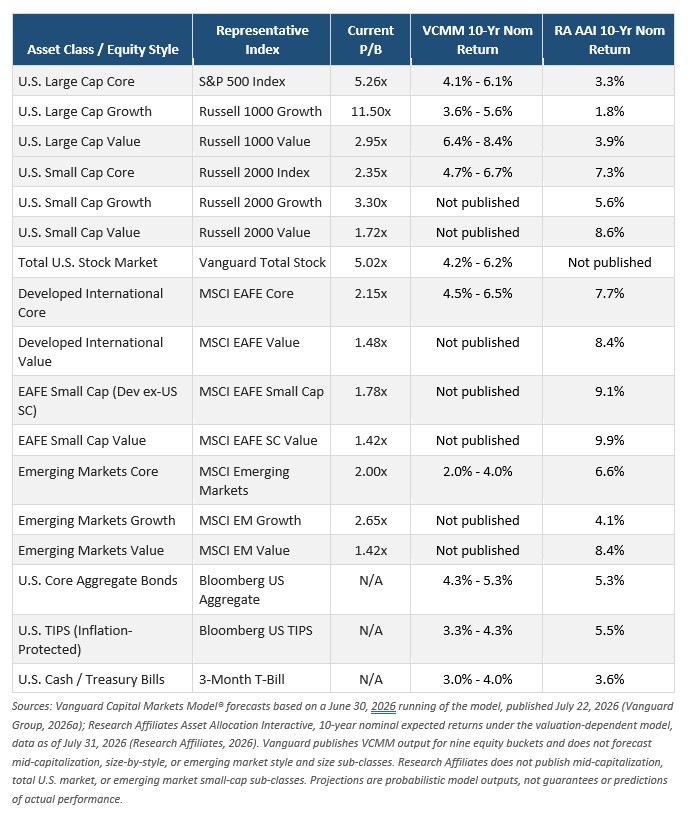
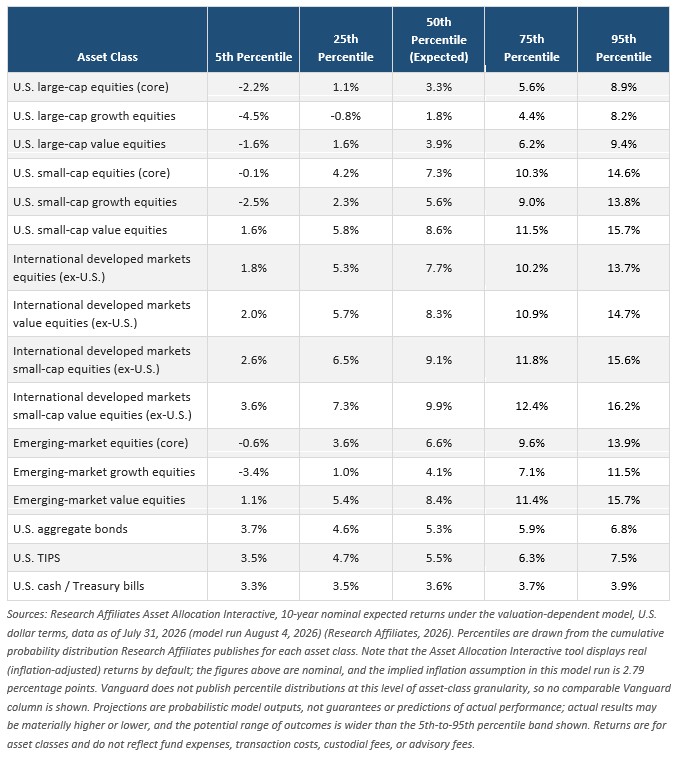
Table 3B: Research Affiliates 10-Year Nominal Return Distributions (2026–2036)

A single expected-return figure conceals how wide the range of plausible outcomes really is. Table 3B reports the full distribution behind the Research Affiliates point estimates in Table 3, using the same July 31, 2026 data. The 50th percentile is the expected 10-year nominal return; the 5th and 95th percentiles bound the central 90% of simulated outcomes. Two features deserve attention. First, the distributions are wide enough that a disappointing decade is entirely possible in every equity asset class – and for U.S. large-cap growth the 25th percentile is negative. Second, the asset classes with the highest expected returns are not merely higher on average; their entire distributions sit further right. International developed small-cap value has a 5th percentile of +3.6%, above the 50th percentile of U.S. large-cap core. That is the practical case for diversifying away from U.S. mega-cap concentration.

Key Insights from Asset Class Dispersion

The comparative data in Table 3 reveals powerful valuation-driven return dispersion across style factors and international regions:

Extreme Premium on U.S. Growth vs. Value. U.S. Large Cap Growth trades at an extraordinary 11.50x P/B, driving Research Affiliates’ 10-year nominal forecast down to 1.8%. By contrast, U.S. Small Cap Value trades at 1.72x P/B, generating a Research Affiliates expected return of 8.6% – a spread of nearly seven percentage points a year. Vanguard does not publish a VCMM forecast for either sub-class. (Vanguard Group, 2026a; Research Affiliates, 2026)
International Developed Small Cap Value Offers High Real Premium. EAFE Small Cap Value trades at 1.42x P/B, with a Research Affiliates projected 10-year nominal return of 9.9%; Vanguard does not publish a VCMM forecast at this level of granularity. Spreading capital into international small-cap value provides fundamental protection against U.S. mega-cap multiple contraction. (Research Affiliates, 2026)
Emerging Markets Value Stands Out as Top Expected Return Asset Class. Emerging Markets Value trades at a modest 1.42x P/B. Driven by strong fundamental earnings growth and low starting entry prices, Research Affiliates forecasts an 8.4% 10-year nominal return. However, the range of possible returns is quite large: at the 90% confidence interval it runs from a 5% probability of an average annualized return below 1.1% to a 5% probability of an average annualized return exceeding 15.7%. (Research Affiliates, 2026)
The Valuation Gap Between U.S. and Non-U.S. Stocks Has Reached a Two-Decade Extreme. These model-based forecasts are corroborated by observable market pricing. On August 10, 2026 the MSCI Emerging Markets Index traded at 9.9 times forward earnings against more than 20 times for the S&P 500 – the first time in at least two decades that emerging market stocks have been valued at less than half the U.S. multiple (Bloomberg News, 2026). In developed markets outside the United States, the MSCI EAFE Value Index returned 33.8% in 2025, its strongest calendar year in more than twenty-five years, and still traded at nearly twice the earnings yield of EAFE growth stocks at October 31, 2025 (Gupta, 2025). Dimensional reports that the MSCI World ex USA and MSCI Emerging Markets indices each returned over 30% in 2025 against 17% for the Russell 3000, while the ten largest S&P 500 constituents grew to over 40% of that index (Dimensional Fund Advisors, 2026). In plain English: the rest of the world is inexpensive relative to the United States by the widest margin most investors alive today have seen – and in 2025 that gap began, at last, to close.

Part VI: Sequence-of-Returns Risk, Rising Equity Glidepaths, and the Bond Tent

For investors transitioning from accumulation to decumulation, sequence-of-returns risk represents the single greatest threat to long-term retirement sustainability (Pfau & Kitces, 2014; Pfau, 2015). When retirees begin taking portfolio distributions during an overvalued market environment, an early market decline permanently impairs the portfolio’s principal base. Because capital is withdrawn to fund living expenses at depressed prices, fewer shares remain to participate in subsequent market recoveries (Kitces, 2014).

Worked Example: Same Returns, in Opposite Order

Maria and David each retire at age 65 with $1,000,000. Each withdraws $50,000 in the first year – 5% of the portfolio – and raises that withdrawal by 3% annually to keep pace with inflation. Over the following twenty-five years each earns exactly the same set of annual returns: five difficult years of –15%, –10%, –5%, +5% and +10%, and twenty years of +8%. Both average 5.8% a year. Both compound at 5.6%. The only difference is the order in which the returns arrive. Maria’s five difficult years come first; David’s come last.

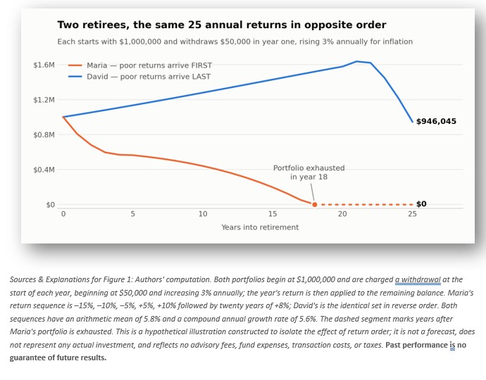
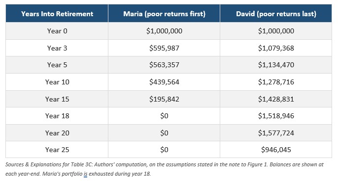
Maria’s portfolio never recovers. Because she must sell shares to fund living expenses while prices are depressed, every early withdrawal permanently removes capital that would otherwise have participated in the rebound. Her balance falls from $1,000,000 to $595,987 by the end of year three. Twenty consecutive years of 8% returns then follow, but too little principal remains for them to work on. Her money runs out in year 18, at age 83.

David’s portfolio compounds for two decades before the same downturn arrives. By the time it does, the balance is large enough to absorb it. He finishes year 25 with $946,045, having drawn inflation-adjusted income for the entire period.

Identical returns. Identical average. Identical withdrawal policy. One retiree is insolvent at 83; the other still holds nearly his original capital at 90.

This is sequence-of-returns risk. For an investor still accumulating, the order of returns does not matter, because nothing is being withdrawn; for a retiree taking distributions, order matters more than average (Pfau & Kitces, 2014). The danger concentrates in the years immediately surrounding retirement, when the portfolio is at its largest and an early loss has the longest time to compound against every later withdrawal (Kitces, 2016). That is why we build a bond tent before retirement, and why we spend from it first.

Table 3C: Portfolio Balance at Selected Years

The Rising Equity Glidepath and Bond Tent Solution

Traditional retirement planning relies on a declining equity glidepath – reducing stock exposure as age advances. However, landmark research by Wade Pfau and Michael Kitces demonstrated that declining glidepaths maximize equity exposure at the precise moment when portfolio size is largest and sequence risk is most severe (Pfau & Kitces, 2014).

Instead, Kitces and Pfau advocate a Rising Equity Glidepath paired with a ‘Bond Tent’:

Building the Bond Tent (Pre-Retirement): In the 5–10 years preceding retirement, investors build a dedicated reserve of short- to intermediate-duration, high-quality fixed income, lowering equity exposure to 30%–40% at the exact retirement date (‘Peak Safety’). (Pfau & Kitces, 2014; Kitces, 2016)
Spending Down the Tent (Early Retirement): During the first 10–15 years of retirement (‘Fragile Decade’), cash withdrawals are funded primarily from the fixed-income buffer. As bonds are spent down, the portfolio’s equity allocation naturally rises toward 60%–70% as sequence risk recedes. (Pfau & Kitces, 2014)

Part VII: Dynamic Withdrawal Strategies & Valuation-Aware Spending

Static withdrawal rules – such as Bengen’s classic “4% rule” – were derived from historical floor scenarios assuming moderate starting valuations (Bengen, 1994). In an environment where the Shiller CAPE exceeds 40, applying a rigid, inflation-adjusted 4% withdrawal rate carries substantial risk of exhaustion for 30+ year retirement horizons (Arnott et al., 2025; Jeske, 2022).

In this table, we compare three approaches to retirement portfolio withdrawals:

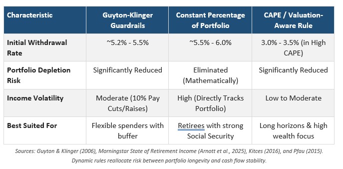
The three approaches differ less in how much risk they carry than in where they place it.

Guyton-Klinger guardrails start high and then defend the portfolio with rules agreed to in advance: if a market decline pushes the current withdrawal rate more than 20% above its starting level, spending is cut by 10%; if a strong market pulls it more than 20% below, spending rises by 10% (Guyton & Klinger, 2006).

The constant-percentage method takes a fixed share of whatever the portfolio is worth each year, so mathematically it can never be exhausted – but a 30% market decline delivers a 30% pay cut in the year a retiree can least absorb one.

The valuation-aware rule runs in the opposite direction, deriving the starting rate from today’s prices rather than from history. Karsten Jeske’s published formulation sets it at 1.75% plus 0.50 divided by the CAPE ratio; at the August 14, 2026 reading of 42.56, that yields roughly 2.9% (authors’ computation from Jeske, 2022) – at or just below the bottom of the range shown above.

What a single row cannot convey is the price of those higher starting rates. Morningstar’s 2025 testing measures the year-to-year variability of the income each method produces across a 30-year retirement: roughly 5% for a fixed, inflation-adjusted withdrawal beginning at 3.9%, about 30% for guardrails beginning at 5.2%, and close to 50% for a constant percentage beginning at 5.6%. Its conclusion is blunt – “the spending strategies that allow for higher initial spending rates generally entail more volatility in cash flows” (Arnott et al., 2025).

No withdrawal rule creates money. Each merely decides who absorbs a bad decade: the portfolio, through a higher risk of exhaustion, or the retiree, through a smaller check. The right choice therefore depends less on the arithmetic than on the household. A retiree whose essential costs – housing, food, insurance, medical care – are already met by Social Security and a pension can tolerate wide swings in what the portfolio contributes, because those swings land on discretionary spending. A retiree whose groceries depend on the portfolio cannot, and should start lower. We therefore recommend setting the initial rate from the client’s guaranteed-income floor and current valuations together, and revisit it annually (Pfau, 2015; Kitces, 2016).

Part VIII: The Three-Bucket Framework

Developed by Harold Evensky (1997) and popularized by Morningstar’s Christine Benz (2024), the Three-Bucket Framework combines time segmentation with disciplined total-return rebalancing to deliver both mathematical resilience and psychological peace of mind:

Bucket 1 (Years 1–2): Near-Term Spending in Cash & Equivalents. Holds 1–2 years of net living expenses in money market funds, Treasury bills, and CDs. Ensures the retiree never faces forced liquidation of equities during market declines. (Benz, 2024; Evensky, 1997)
Bucket 2 (Years 3–10): Intermediate-Term Fixed Income. Holds 7–8 years of cash flow needs in high-quality short- and intermediate-term bonds and TIPS. Acts as a bridge, generating steady yield and refilling Bucket 1 during equity downturns. (Benz, 2024)
Bucket 3 (Years 11+): Long-Term Factor-Tilted Growth. Holds globally diversified equities tilted toward value, size, and profitability factors. Because Bucket 3 assets are not needed for at least a decade, they have ample runway to recover from market corrections. (Benz, 2024; Fama & French, 2018)

The framework’s principal contribution is behavioral, and that is not a small thing. Evensky designed the cash reserve precisely so that a retiree would never be compelled to sell equities into a decline (Evensky, 1997), and Benz has been consistently candid that the buckets’ central function is to make a portfolio’s purpose visible: a client who can see two years of groceries sitting in cash and a decade of income sitting in bonds finds it markedly easier to leave Bucket 3 untouched through a bear market (Benz, 2024). Part X of this report documents what abandoning a plan at the wrong moment actually costs – missing only the ten best trading days across fifteen international markets reduced terminal wealth by an average of 50.8% (Estrada, 2008). Measured against a loss of that magnitude, a structure that helps a client stay seated earns its place on the merits.

Whether it improves long-term returns is a separate question, and the candid answer is that it does not. A bucket structure is an asset allocation wearing different labels: a retiree holding two years of spending in cash, eight years in bonds, and the remainder in equities owns the same portfolio as one holding roughly 8% cash, 32% bonds, and 60% equities and rebalancing on a schedule. The return comes from the mix, not from the naming. Where the two genuinely diverge is the standing cash reserve, and there the difference runs against bucketing. On the Research Affiliates estimates in Table 3, cash is expected to return 3.6% annually over the coming decade against 5.3% for aggregate bonds. Holding two years of a 4% withdrawal – about 8% of the portfolio – permanently in cash rather than bonds therefore costs roughly 0.14 percentage points a year, compounding to approximately 4% less wealth over thirty years (authors’ computation from Research Affiliates, 2026). Formal testing reaches the same conclusion, and more sharply. Javier Estrada compared three bucket strategies against eleven static, periodically rebalanced allocations across 21 countries and 86 rolling 30-year retirement periods drawn from 1900 through 2014. In U.S. data the static 60–70% equity allocations failed in 0% to 1.2% of periods against 3.5% to 4.7% for the bucket strategies, and Estrada concluded that “simple static strategies, which by definition involve periodic rebalancing, clearly outperform bucket strategies” on every metric he tested (Estrada, 2019). We therefore use the framework because a plan a client will actually keep is worth more than a marginally more efficient plan he abandons in a panic – not because the buckets add return.

Part IX: Multi-Factor Investing & Factor Diversification as Risk Management

Factor investing is frequently misunderstood as an aggressive return-seeking strategy. In reality, tilting equities toward empirically documented academic risk factors – Market (MKT), Size (SMB), Value (HML), Profitability (RMW), and Investment (CMA) from the Fama-French five-factor model, together with Momentum (MOM) from Carhart (1997) – can serve as a powerful risk-management tool that reduces overconcentration in richly valued mega-cap growth stocks (Fama & French, 1993, 2015, 2018; Carhart, 1997).

The cautionary precedent is the 2000–2009 ‘Lost Decade.’ Following the late-1990s technology bubble peak, the cap-weighted S&P 500 delivered a negative -0.95% annualized total return over 10 years (Dimensional Fund Advisors, 2020). In stark contrast, factor-tilted equities flourished: U.S. Small Cap Value delivered +7.7% annualized, U.S. Mid-Cap Value delivered +7.2% annualized, and International Small Cap produced robust positive returns (Dimensional Fund Advisors, 2020). Diversifying across academic factors may cushion portfolios against high-valuation unwinds.

However, as we’ve noted above, unlike early 2000, the overvaluation we observe today is broader than U.S. growth alone – though, as Table 1B notes, the independent academic series does not corroborate that extreme overvaluation reading for the U.S. small-cap value segment. French’s series is constructed from CRSP data with NYSE breakpoints and is U.S.-only; no equivalent foreign series was available for direct comparison.

Part X: Tactical Asset Allocation and Market Timing – Is It Justified to Grow More Conservative in an Extraordinarily Expensive Market?

Everything set out in Parts I through IX leads a thoughtful client to one question, and it is usually asked in plain words: if stocks are this expensive, why not simply own fewer of them until they are cheaper? The question deserves a serious answer rather than a slogan. It is not foolish. It follows logically from the evidence, and some respected academic work supports a version of it.

The practice of deliberately shifting a portfolio away from its long-term targets in response to a forecast is called tactical asset allocation, or, less politely, market timing. The two terms describe the same activity at different levels of formality: tactical asset allocation generally means modest, rule-based shifts among asset classes, while market timing usually connotes larger, discretionary moves in and out of the market. Both rest on the same premise – that an investor can identify in advance when one asset class will outperform another, and act on that knowledge profitably after costs and taxes.

This Part reviews what the academic literature actually establishes, explains why a tactical shift requires two correct decisions rather than one, quantifies what a move toward a more conservative portfolio surrenders in expected return, and closes with the distinction we believe fiduciary advisers must draw between changing a portfolio because of a forecast and changing it because a client’s circumstances have changed.

What the Academic Evidence Establishes

The weight of the peer-reviewed evidence is unfavorable to tactical asset allocation as it is actually practiced. Five findings are worth a client’s attention.

Valuation-based switching rules do not survive honest testing. Kenneth Fisher and Meir Statman tested market-timing rules based on price-to-earnings ratios and dividend yields across the period 1871 to 2002, examining every critical price-to-earnings threshold from 5 to 40 and dividend yield thresholds from 1.00% to 10.50%. Not one of the price-to-earnings rules beat buy-and-hold: the best of them accumulated $60,628 against $67,672 for simply staying invested. One dividend-yield rule did beat buy-and-hold, accumulating $98,289 – but it was identified only in hindsight, by searching the same data it was then tested on. Their conclusion was that no widely available valuation measure is a reliable timing guide, and that successful timing requires insights beyond those such measures contain (Fisher & Statman, 2006).
The broader class of return-prediction models fails out of sample. Amit Goyal and Ivo Welch conducted the definitive examination of this question, testing roughly fifteen predictor variables – dividend-price ratios, earnings-price ratios, book-to-market, interest rate spreads, corporate issuing activity, inflation, and others – at annual, five-year, and monthly frequencies. Most models were not statistically significant even in sample, and most performed poorly out of sample for more than thirty years. Their conclusion was stated without hedging: these models ‘would not have helped an investor with access only to available information to profitably time the market’ (Goyal & Welch, 2008).
Professional managers paid to do this have not done it well. Vanguard evaluated 24 U.S. stock-and-bond tactical asset allocation mutual funds over January 1995 through December 2009 and found average monthly excess return of 0.08% with a t-statistic of 0.16 – statistically indistinguishable from zero – and an average information ratio of 0.02. The authors calculated that break-even trading costs ranged from 0.7% to 4.7% annually depending on turnover, and concluded that while implementing tactical allocation ‘is often portrayed as simple, it is actually very difficult’ (Stockton & Shtekhman, 2010). Morningstar’s later examination was harsher. Of 34 tactical allocation funds of funds identified in April 2013, only 12 survived the following decade; not one of the 12 survivors produced a higher return or a higher Sharpe ratio than a plain U.S. 60/40 portfolio, which returned roughly 7.5% annually against 2.3% for the average tactical fund. Thirty of the 34 would have done better had their managers simply stopped trading, the average shortfall from trading being about 4.4% a year (Ptak, 2023).
A very small number of days produce most of the return, and they cannot be identified in advance. Javier Estrada examined 160,278 trading days across 15 international equity markets spanning 627 market-years. Missing only the ten best days reduced terminal wealth by an average of 50.8% across markets; missing the best 100 days – under 1% of all trading days – reduced it by 97.7%. In the Dow Jones Industrial Average from 1900 to 2006, $100 grew to $25,746, but missing the ten best days cut that to $9,008. Estrada acknowledged that avoiding the worst days is even more valuable than capturing the best ones; his point is that neither set can be identified beforehand, which makes timing ‘a highly improbable’ route to excess return (Estrada, 2008).
The behavioral cost of trading is real, though smaller than commonly claimed. Candor requires reporting a correction here. Morningstar’s widely cited “Mind the Gap” studies have estimated that poor timing costs fund investors roughly 1.2% a year, or about 15% of the returns their own funds earned. Examining the identical dataset, Fulkerson, Jordan, Riley, and Yan concluded in the Financial Analysts Journal that the true cost of poor timing is approximately 0.10% per year – roughly one-twelfth of the headline figure – and that the Return Gap metric conflates several effects into a single number that overstates behavioral cost (Fulkerson et al., 2026). We cite the corrected figure rather than the more dramatic one. The case against tactical allocation does not require exaggeration.

The Evidence on the Other Side, Stated Fairly

It would be intellectually dishonest to present only one side. Serious researchers have found that valuation carries real information, and that disciplined, moderate use of it can help. Three findings deserve equal weight.

Starting valuations genuinely do predict long-horizon returns. This is not in dispute, and it is the foundation of this entire report. John Campbell and Robert Shiller established the relationship between valuation ratios and subsequent long-horizon returns (Campbell & Shiller, 1988; Shiller, 2015). Michael Kitces quantifies the horizon dependence precisely: the correlation between the cyclically adjusted earnings yield and subsequent returns is only 0.23 at one year, rises to 0.53 at ten years, and peaks at roughly 18 years for real returns. The information is real; it simply arrives on a timescale that is useless for trading (Kitces, 2014).
Modest, rules-based valuation tilts can improve risk-adjusted outcomes – modestly. Cliff Asness, Antti Ilmanen, and Thomas Maloney examined this question directly in a paper aptly titled ‘Market Timing: Sin a Little.’ Over 1900 to 2015, buy-and-hold produced a Sharpe ratio of 0.38; pure contrarian value timing produced 0.37 – that is, no improvement at all. Combining value with momentum signals raised it to 0.43, an improvement the authors themselves characterize as modest. They also catalogue the reasons for caution: valuations have drifted persistently higher over the past six decades, producing chronic underinvestment signals; a century of data contains few genuinely independent long-horizon observations; and selection and data-mining biases are, in their words, endemic to market timing studies (Asness et al., 2017).
In retirement portfolios specifically, valuation-responsive allocation has tested well. This is the most directly relevant finding for our clients. Michael Kitces and Wade Pfau tested valuation-based asset allocation over U.S. data from 1871 to 2013 across 30-year retirements, using a rule adapted from Graham and Dodd: hold a neutral 45% equity allocation when the cyclically adjusted price-to-earnings ratio sits between two-thirds and four-thirds of its rolling historical median, raise equities to 60% when stocks are undervalued, and reduce to 30% when they are overvalued. The valuation-based approach produced results comparable to or slightly better than both static allocations and rising equity glide paths across the range of starting conditions, and the authors concluded that the optimal retirement allocation does appear contingent on market valuation (Kitces & Pfau, 2015). Separately, Pfau found that valuation-based timing rules delivered returns comparable to a 100% stock buy-and-hold strategy with substantially less risk, while cautioning that extreme all-in, all-out versions fail to protect investors during the extended periods when valuations depart from historical norms (Pfau, 2011).

Read together, this literature supports a narrow conclusion rather than a broad one. Modest, pre-committed, rule-based responses to valuation – of the kind Kitces and Pfau tested, where the equity allocation moves within a band of 30% to 60% according to a rule written down in advance – have empirical support. Discretionary decisions to leave the market because it feels dangerously expensive do not. The difference between those two activities is the subject of the next two sections.

Why Tactical Asset Allocation Requires Two Correct Decisions, Not One

The central practical difficulty with reducing equity exposure in an expensive market is one that clients rarely consider when they raise the idea, and that its advocates rarely address. Getting out is only half the problem. A tactical shift is not complete until the portfolio has been restored to its target, which means every tactical decision is really two decisions – and both must be right.

The first decision is when to reduce. To profit, the investor must be correct not merely that equities are expensive – which Parts I and II establish beyond reasonable argument – but that equities will underperform the safer asset over the specific period during which the money is actually parked. Those are different claims. A market can remain expensive, and keep rising, for a very long time, and valuation carries almost no information about the coming twelve months: the correlation between the cyclically adjusted earnings yield and the next year’s return is only 0.23 (Kitces, 2014). An investor who acts on a valuation signal is therefore making a claim about a period whose length he cannot know in advance.

The second decision is when to restore. This one is harder, and it is the decision that actually destroys portfolios. Re-entry must occur when conditions feel worst – amid falling prices, unfavorable headlines, and the fresh memory of having been right. Worse, an investor who left the market at a CAPE ratio of 42.56 must decide what reading justifies returning. A 25% decline would leave the ratio near 32, still roughly twice its long-run median of 16.11, but closer to a more recent 20-year or 25-year median. A rule that waits for fair value may never trigger: as Asness, Ilmanen, and Maloney document, valuations have drifted higher for six decades, generating persistent signals to stay underinvested throughout a period in which equities delivered substantial returns (Asness et al., 2017). The tactical investor who cannot answer the re-entry question in advance has not made a temporary allocation shift. He has made a permanent one, and simply does not know it yet.

The accuracy required is high. William Sharpe examined this arithmetic in 1975 and concluded that an investor switching between stocks and cash should expect to be right at least seven times out of ten before the attempt is worth making (Sharpe, 1975, as summarized in Blanchett, 2011). David Blanchett revisited the question with modern cost and tax assumptions and found that a tactical strategy must be right approximately 66% of the time before taxes, and approximately 70% of the time after taxes, merely to match a static allocation on a risk-adjusted basis; his after-tax analysis showed tactical strategies trailing by 50 to 90 basis points a year, largely because gains are realized at short-term rates and compounding is interrupted (Blanchett, 2011).

Table 4A: The Two Decisions a Tactical Shift Requires

Table 4A sets out the two decisions side by side, together with the consequence of getting each one wrong.

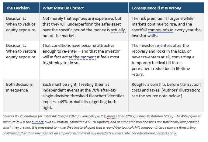
The Arithmetic of a Surrendered Risk Premium

Suppose an investor makes both decisions correctly. There remains a third problem, and it is the one least often examined: the cost of waiting. Moving toward a more conservative portfolio does not merely reduce risk. It surrenders compensation – and not a single premium, but several at once.

A portfolio that moves from diversified global equities into high-quality bonds gives up the equity risk premium. If it also abandons a small-cap and value tilt of the kind described in Part IX, it gives up the size and value premiums as well (Fama & French, 1993, 2018). If it moves further, from intermediate bonds into Treasury bills, it additionally surrenders the term premium; if it moves from corporate credit into Treasuries, the credit premium. Each of these is small in any given year and decisive over a decade. Across 1900 through 2025 – 126 years – U.S. equities returned 6.6% a year in real (inflation-adjusted) terms against 1.6% for bonds and 0.5% for Treasury bills, a premium of roughly five percentage points a year over U.S. Treasury bonds and six percentage points over U.S. Treasury bills (Dimson et al., 2026).

Here, however, the honest answer becomes more interesting than the conventional one, because the size of the premium being surrendered today depends entirely on which equities are being sold. Table 4B applies this report’s own forward-looking estimates to the question.

Table 4B: What Moving Conservative Surrenders, Using This Report’s Own Forecasts

Table 4B restates selected forecasts from Table 3 and expresses each as a premium over, or shortfall against, the U.S. aggregate bond market.

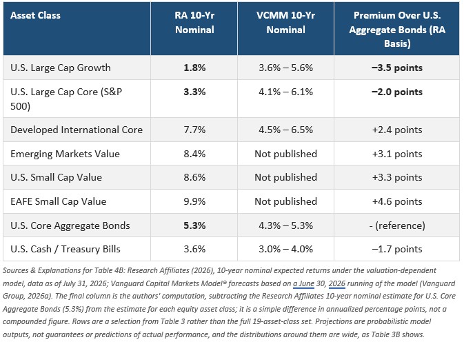
Table 4B carries an uncomfortable implication for both sides of this argument. On Research Affiliates’ numbers, an investor who sells the S&P 500 and buys the aggregate bond market surrenders nothing at all – he picks up two percentage points a year of expected return, and reduces volatility while doing so. If the only question were whether to abandon U.S. mega-cap growth, the arithmetic would favor doing exactly that.

But that is not the portfolio our clients own, and it is not the portfolio this report recommends. A globally diversified, value- and size-tilted equity allocation of the kind described in Parts IX and XI carries a Research Affiliates expected return in the range of roughly 8% to 9% nominal – some two-and-a-half to three-and-a-half percentage points above bonds and four-and-a-half to five-and-a-half points above cash. That is the premium actually at stake, and it is substantial.

Consider what surrendering it costs. An investor who moves from a diversified equity portfolio expected to return 8% into bonds expected to return 5.3% gives up roughly 2.6 percentage points of compounded annual growth. Over ten years, the equity portfolio ends approximately 29% larger; put the other way, the conservative portfolio finishes with about 78 cents for every dollar the equity portfolio produces (authors’ computation from Research Affiliates, 2026). This shortfall accrues quietly, every year, whether or not the feared decline ever arrives.

The break-even calculation is more revealing still. An investor who moves that same portfolio to Treasury bills expected to return 3.6% falls behind by roughly 4.2 percentage points a year. After five years the equity portfolio is ahead by about 23%, which means the market would have to fall roughly 19% from its then-prevailing level merely to restore the waiting investor to even – before transaction costs, before taxes, and before the practical difficulty of buying into a 19% decline (authors’ computation from Research Affiliates, 2026). This is why the loss of a risk premium is so hard to recover: the cost of waiting is certain, recurring, and compounds, while the hoped-for decline is uncertain, one-time, and must be acted upon at the moment of maximum fear.

Taxes deepen the problem in taxable accounts. Blanchett’s after-tax modeling found tactical strategies trailing static allocations by 50 to 90 basis points a year, primarily because appreciated positions must be sold to implement the shift, triggering capital gains that would otherwise have been deferred indefinitely (Blanchett, 2011). An investor sitting on large embedded gains after a multi-year bull market faces the highest tax cost precisely when the temptation to sell is strongest.

So, is De-Risking Ever Justified? The Fiduciary Distinction

Our answer is yes – but for a reason that has nothing to do with forecasting, and that requires only one decision rather than two.

There is a categorical difference between changing a portfolio because of a prediction about markets and changing it because something about the client has changed. The first is market timing, and the evidence above should make any fiduciary cautious about it. The second is financial planning, and it is not market timing at all – even when the two produce identical trades.

The distinction matters because valuation legitimately changes what a portfolio can be asked to do. Kitces demonstrates that while the cyclically adjusted earnings yield correlates only 0.23 with returns over the following year, the Shiller price-to-earnings ratio correlates −0.74 with sustainable withdrawal rates – an extraordinarily strong inverse relationship, meaning that the more expensive the market, the less a retiree can safely spend (Kitces, 2014). Valuation, in other words, is nearly useless for deciding when to trade and enormously useful for deciding how much a retiree can safely spend, whether delaying Social Security is worthwhile, and whether a pension should be taken as an annuity or a lump sum. Those are decisions whose consequences unfold over exactly the horizon on which valuation carries information.

Applying that logic, we regard a shift toward a more conservative allocation as defensible in four circumstances, none of which requires a forecast:

The plan no longer survives its own stress test. If a valuation-aware analysis shows that a household’s spending plan fails under the lower return distributions documented in Tables 3 and 3B, the portfolio is carrying more equity risk than the plan can absorb. Reducing equity is then a response to an identified planning shortfall, not a market call, and it should be made permanently rather than tactically (Kitces, 2014; Arnott et al., 2025).
The client is inside the fragile decade. For investors in the five to ten years before retirement and the first ten to fifteen years after it – the window Part VI calls the fragile decade – the bond tent described in Part VI deliberately lowers equity exposure to 30%–40% at the retirement date and allows it to rise thereafter. This is a pre-committed, age-based schedule that would be followed at any valuation level. It happens to reduce equity exposure today, but it would have done so in 2009 as well (Pfau & Kitces, 2014; Kitces, 2016).
The reduction follows a rule written down in advance. The valuation-responsive approach Kitces and Pfau tested – moving within a 30% to 60% equity band according to where the cyclically adjusted price-to-earnings ratio sits relative to its rolling historical median – has empirical support precisely because it is mechanical. It specifies the re-entry condition at the same moment it specifies the exit, which collapses the two-decision problem into a single decision made in advance, while calm (Kitces & Pfau, 2015). What it does not permit is discretion in the moment. Two cautions apply. Their rule is measured against a rolling historical median rather than a fixed one, precisely so that the drift Asness and colleagues document does not lock an investor out permanently; and where its prescription conflicts with the age-based bond tent schedule set out in Part VI, the Part VI schedule governs in our practice. We cite the Kitces-Pfau results as evidence that valuation-responsive allocation can be done responsibly, not as a rule we apply mechanically to client portfolios.
The client’s true risk tolerance was overstated. If a client would abandon the plan during a 40% decline, an allocation that assumes otherwise is not prudent regardless of expected return. A portfolio the client can actually hold through a bear market is superior to a theoretically optimal one that is sold at the bottom, and the evidence in this Part on the cost of poorly timed exits is precisely why (Estrada, 2008; Ptak, 2023).

What we do not do is reduce equity exposure because a valuation measure is high and it feels prudent to act. That is the discretionary version, it requires two correct forecasts, and it is the version the literature reviewed above does not support.

One clarification is owed to readers of the Executive Summary and of Part XI, both of which discuss Berkshire Hathaway’s substantial cash position. We cite Berkshire as an illustration of holding liquidity sufficient to meet near-term obligations without being forced to sell at depressed prices – the discipline described in Part XI – and not as an endorsement of building cash because a valuation measure is elevated. Berkshire is an operating company with insurance liabilities and an opportunistic acquisition mandate; a retiree drawing income from a diversified portfolio is not in that position, and should not infer from Berkshire’s balance sheet that a forecast-driven cash build is prudent for a household.

It is worth naming what this report already does with its valuation findings, because it is not nothing. Rather than reducing total equity exposure, our approach is to reallocate within it – away from the U.S. mega-cap growth stocks that Table 4B shows carry a negative expected premium over bonds, and toward the international, small-cap, and value segments that carry premiums of roughly two to four-and-a-half points. That response harvests the information in the valuation data without surrendering the equity risk premium, and it requires no forecast about timing whatsoever. Systematic rebalancing, described in Part XI, accomplishes much of it automatically. Individual client allocations are set in light of each household’s circumstances.

In plain English: the honest answer to ‘should I get more conservative because the market is expensive?’ is that you should get more conservative if your plan needs you to, if you are approaching or in early retirement, or if you know you could not sit through a severe decline. You should not do it because you or we believe stocks are due to fall. The first set of reasons requires one decision, made calmly, and it stays made. The second requires two decisions, both made under pressure, and the research says that most people – professionals very much included – get at least one of them wrong.

Part XI: Practical Fiduciary Guidance & Implementation Framework

To translate academic research into actionable client outcomes, advisers at Scholar Financial implement the following core portfolio construction principles:

Rebalance Systematically (‘Buy Low, Sell High’). Enforce strict target allocation rebalancing bands. Systematically trim appreciated asset classes during market surges and reallocate capital into out-of-favor, lower-valued segments. (Kitces, 2014)
Embrace Global and Style Diversification. Overcome home-country bias by allocating meaningful equity weightings to Developed Markets Small Cap Value, Emerging Markets Value, and Emerging Markets Small Cap Value, where forward expected returns are substantially higher. (Research Affiliates, 2026; Vanguard Group, 2026a)
Maintain Cash Discipline without Market Timing. Follow the fiduciary model illustrated by Berkshire Hathaway: hold sufficient liquidity to cushion near-term liabilities (in a separate cash reserve account that is not managed, and through an asset allocation to short-term high quality bonds within the managed portfolio), but remain fully disciplined to long-term target asset allocations rather than attempting binary market timing. (Berkshire Hathaway, 2026; The Motley Fool, 2026)

About the Authors

Ron A. Rhoades, JD, CFP^® is an Associate Professor of Finance at the Gordon Ford College of Business, Western Kentucky University. He also serves as a financial advisor at Scholar Financial, a practice within XY Investment Solutions LLC. With a background as both an attorney and a CERTIFIED FINANCIAL PLANNER™ professional, Ron is a nationally recognized authority on the fiduciary duties of financial advisors.

Chris Brown, Ph.D., CFP^® is a faculty member in the Department of Finance at the Gordon Ford College of Business, Western Kentucky University, and a financial advisor at Scholar Financial, a practice within XY Investment Solutions, LLC. He holds the CERTIFIED FINANCIAL PLANNER™ designation and a Ph.D. in Finance. His research and teaching focus is on behavioral finance, retirement planning, and evidence-based investment strategies.

Scholar Financial is a fee-only, fiduciary practice within XY Investment Solutions, LLC.

Contact: AdvisorInfo@ScholarFinancial.com.

Disclosures & Legal Disclaimers

The opinions expressed in this commentary are solely those of the individual author and do not necessarily reflect the views or opinions of XYIS. These opinions are based on information available at the time of posting and are subject to change without notice. Information is based on reliable data available as of August 14, 2026, but accuracy cannot be guaranteed. Nothing herein constitutes individualized investment, tax, or legal advice. Forward-looking return estimates are model outputs derived from third-party tools (Vanguard VCMM and Research Affiliates AAI) and carry wide potential return distributions. Past performance does not guarantee future results.

XYIS does not commit to updating any posted positions or commentary to reflect subsequent developments. While the information and reasoning used to form these opinions are believed to be from reliable sources, XYIS does not verify this information, and no guarantee is provided regarding its accuracy, completeness, or validity. XYIS disclaims any and all liability for actions taken or not taken based on the content of this article. No warranty, express or implied, is given in connection with the content provided.

Advisory services are offered through XYPN Sapphire and its various IAR brands under which it operates. XYPN Sapphire is an SEC registered investment adviser. For additional disclosure and privacy information, please visit XYPNSapphire.com/disclosures.

Sources

AQR Capital Management. (2025, December 31). 2026 capital market assumptions for major asset classes (Alternative Thinking, 2026 Issue 1). https://www.aqr.com/Insights/Research/Alternative-Thinking/2026-Capital-Market-Assumptions-for-Major-Asset-Classes

Arnott, A. C., Benz, C., Kephart, J., & Guo, T. (2025, December 3). The state of retirement income: 2025. Morningstar. https://www.morningstar.com/business/insights/research/the-state-of-retirement-income

Asness, C. S., Ilmanen, A., & Maloney, T. (2017). Market timing: Sin a little. Journal of Investment Management, 15(3), 23–40. https://www.aqr.com/-/media/AQR/Documents/Insights/White-Papers/Market-Timing-Sin-a-Little.pdf

Bain & Company. (2025, September 23). $2 trillion in new revenue needed to fund AI’s scaling trend. https://www.bain.com/about/media-center/press-releases/20252/

Barclays. (2024). Artificial intelligence software monetization and hyperscaler CapEx trends. Barclays Equity Research.

Bengen, W. P. (1994). Determining withdrawal rates using historical data. Journal of Financial Planning, 7(4), 171–180.

Benz, C. (2024). How to retire: 20 lessons for a happy, successful, and wealthy retirement. Harriman House.

Berkshire Hathaway Inc. (2026). Form 10-Q for the quarterly period ended June 30, 2026. U.S. Securities and Exchange Commission. https://www.sec.gov/Archives/edgar/data/1067983/000119312526341032/brka-20260630.htm

Blanchett, D. M. (2011, February). Is buy and hold dead? Exploring the costs of tactical reallocation. Journal of Financial Planning, 24(2). https://www.financialplanningassociation.org/article/journal/FEB11-buy-and-hold-dead-exploring-costs-tactical-reallocation

Bloomberg News. (2026, August 10). Emerging-market stock valuations sink below half of S&P 500’s. Bloomberg, via Yahoo Finance. https://finance.yahoo.com/markets/world-indices/articles/emerging-market-stock-valuations-sink-115217478.html

Buffett, W. E., & Loomis, C. J. (2001, December 10). Warren Buffett on the stock market. Fortune. https://fortune.com/2001/12/10/warren-buffett-stock-market/

Butters, J. (2026, August 7). S&P 500 earnings season update: August 7, 2026. FactSet Research Systems. https://insight.factset.com/sp-500-earnings-season-update-august-7-2026

Cahn, D. (2024, June 20). AI’s $600B question. Sequoia Capital. https://www.sequoiacap.com/article/ais-600b-question/

Cambridge Associates. (2025, December 3). 2026 outlook: Public equity views. https://www.cambridgeassociates.com/insight/2026-outlook-public-equity-views/

Campbell, J. Y., & Shiller, R. J. (1988). Stock prices, earnings, and expected dividends. The Journal of Finance, 43(3), 661–676. https://doi.org/10.1111/j.1540-6261.1988.tb04598.x

Carhart, M. M. (1997). On persistence in mutual fund performance. The Journal of Finance, 52(1), 57–82. https://doi.org/10.1111/j.1540-6261.1997.tb03808.x

Charles Schwab. (2026, January 27). Are stocks overvalued? 5 indicators to watch. https://www.schwab.com/learn/story/are-stocks-overvalued-5-indicators-to-watch

Current Market Valuation. (2026). Buffett indicator valuation model. Retrieved August 14, 2026, from https://www.currentmarketvaluation.com/models/buffett-indicator.php

Damodaran, A. (2026, March). The price of risk: An equity risk premium monologue! Musings on Markets. https://aswathdamodaran.blogspot.com/2026/03/the-price-of-risk-equity-risk-premium.html

DeepSeek-AI. (2024). DeepSeek-V3 technical report (arXiv:2412.19437). arXiv. https://arxiv.org/abs/2412.19437

DeepSeek. (2026). Models and pricing. Retrieved August 14, 2026, from https://api-docs.deepseek.com/quick_start/pricing

Dimensional Fund Advisors. (2020, February 3). A tale of two decades: Lessons for long-term investors. https://www.dimensional.com/us-en/insights/a-tale-of-two-decades

Ahn, B. H., & Saito, N. (2023, April 10). Assessing alternative value metrics. Dimensional Fund Advisors. https://www.dimensional.com/us-en/insights/assessing-alternative-value-metrics

Dimensional Fund Advisors. (2026, April 23). Insights from Dimensional’s Portfolio Consulting Group: Q1 2026 market themes. https://www.dimensional.com/us-en/insights/insights-from-dimensionals-portfolio-consulting-group-q1-2026-market-themes

Dimson, E., Marsh, P., & Staunton, M. (2026). Global investment returns yearbook 2026: Summary edition. UBS. https://www.ubs.com/content/dam/assets/wm/static/cio/documents/giry2026-summary-public.pdf

Estrada, J. (2008). Black swans and market timing: How not to generate alpha. The Journal of Investing, 17(3), 20–34. https://blog.iese.edu/jestrada/files/2012/06/BlackSwans.pdf

Estrada, J. (2019). The bucket approach for retirement: A suboptimal behavioral trick? The Journal of Investing, 28(5). https://blog.iese.edu/jestrada/files/2019/07/BucketApproach.pdf

Evensky, H. R. (1997). Wealth management: The financial advisor’s guide to investing and managing your client’s assets. McGraw-Hill.

Fama, E. F., & French, K. R. (1993). Common risk factors in the returns on stocks and bonds. Journal of Financial Economics, 33(1), 3–56. https://doi.org/10.1016/0304-405X(93)90023-5

Fama, E. F., & French, K. R. (2015). A five-factor asset pricing model. Journal of Financial Economics, 116(1), 1–22. https://doi.org/10.1016/j.jfineco.2014.10.010

Fama, E. F., & French, K. R. (2018). Choosing factors. Journal of Financial Economics, 128(2), 234–252. https://doi.org/10.1016/j.jfineco.2018.02.012

Fisher, K. L., & Statman, M. (2006). Market timing in regressions and reality. The Journal of Financial Research, 29(3), 293–304. https://doi.org/10.1111/j.1475-6803.2006.00179.x

French, K. R. (2026). Current research returns [Data set]. Kenneth R. French Data Library, Tuck School of Business at Dartmouth College. Retrieved August 14, 2026, from https://mba.tuck.dartmouth.edu/pages/faculty/ken.french/data_library.html

Fulkerson, J. A., Jordan, B. D., Riley, T. B., & Yan, Q. (2026). Bad timing does not cost investors 15% of their funds’ returns: An examination of Morningstar’s “Mind the Gap” study. Financial Analysts Journal, 82(3). https://doi.org/10.1080/0015198X.2026.2657253

Galloway, S. (2026, July 17). 1999.AI. No Mercy / No Malice. https://www.profgmedia.com/p/no-mercy-no-malice-1999ai

Gartner. (2026, July 20). Gartner forecasts worldwide AI platforms and models market to grow 63% in 2026. https://www.gartner.com/en/newsroom/press-releases/2026-07-20-gartner-forecasts-worldwide-ai-platforms-and-models-market-to-grow-63-percent-in-2026

Goldman Sachs Research. (2024, June 25). Gen AI: Too much spend, too little benefit? (Top of Mind). Goldman Sachs. https://www.goldmansachs.com/insights/top-of-mind/gen-ai-too-much-spend-too-little-benefit

Goldman Sachs Research. (2025, December 22). Macro outlook 2026: Sturdy growth, stagnant jobs, stable prices. Goldman Sachs. https://www.goldmansachs.com/insights/goldman-sachs-research/macro-outlook-2026-sturdy-growth-stagnant-jobs-stable-prices

Goldman Sachs Research. (2026, August 7). Global AI investment is forecast to exceed $1 trillion in 2026. Goldman Sachs. https://www.goldmansachs.com/insights/articles/global-investment-is-forecast-to-exceed-1-trillion-in-2026

Goyal, A., & Welch, I. (2008). A comprehensive look at the empirical performance of equity premium prediction. The Review of Financial Studies, 21(4), 1455–1508. https://academic.oup.com/rfs/article-abstract/21/4/1455/1565737

Guo, D., Yang, D., Zhang, H., Song, J., & DeepSeek-AI. (2025). DeepSeek-R1 incentivizes reasoning in LLMs through reinforcement learning. Nature, 645(8081), 633–638. https://doi.org/10.1038/s41586-025-09422-z

Gupta, R. (2025, December 11). International value has outshone US growth. MSCI Inc. https://www.msci.com/research-and-insights/blog-post/international-value-has-outshone-us-growth

GuruFocus. (2026). Shiller excess CAPE yield for the S&P 500. Retrieved August 14, 2026, from https://www.gurufocus.com/economic_indicators/4530/shiller-excess-cape-yield-for-the-sp-500

Guyton, J. T., & Klinger, W. J. (2006). Decision rules and maximum initial withdrawal rates. Journal of Financial Planning, 19(3), 48–58.

Hussman, J. P. (2026, June 1). Record extremes, alternative investments, and the hippo. Hussman Funds. https://www.hussmanfunds.com/comment/mc260601/

Ilmanen, A. (2011). Expected returns: An investor’s guide to harvesting market rewards. John Wiley & Sons.

Investment Company Institute. (2026). Money market fund assets. https://www.ici.org/research/stats/mmf

J.P. Morgan Asset Management. (2025, October 20). J.P. Morgan releases 2026 long-term capital market assumptions [Press release]. https://am.jpmorgan.com/us/en/asset-management/institutional/about-us/media/press-releases/jp-morgan-releases-2026-long-term-capital-market-assumptions/

Jeske, K. (2022, October 12). The 4% rule works again! An update on dynamic withdrawal rates based on the Shiller CAPE – SWR series part 54. Early Retirement Now. https://earlyretirementnow.com/2022/10/12/dynamic-withdrawal-rates-based-on-the-shiller-cape-swr-series-part-54/

Kitces, M. E. (2014, August 6). Shiller PE: Bad market timing, good retirement planning. Nerd’s Eye View. https://www.kitces.com/blog/shiller-cape-market-valuation-terrible-for-market-timing-but-valuable-for-long-term-retirement-planning/

Kitces, M. E. (2016, October 5). The portfolio size effect and using a bond tent to navigate the retirement danger zone. Nerd’s Eye View. https://www.kitces.com/blog/managing-portfolio-size-effect-with-bond-tent-in-retirement-red-zone/

Kitces, M. E., & Pfau, W. D. (2015, March). Retirement risk, rising equity glide paths, and valuation-based asset allocation. Journal of Financial Planning, 28(3), 38–48. https://www.financialplanningassociation.org/article/journal/MAR15-retirement-risk-rising-equity-glide-paths-and-valuation-based-asset

Bank of America Global Research. (2026, July). Global Fund Manager Survey, July 2026.

Masturzo, J., & Kunz, B. (2017, June). Forecasting asset and portfolio expected returns [Webinar]. Research Affiliates. https://www.researchaffiliates.com/insights/multimedia/623-webinar-replay-forecasting-asset-and-portfolio-expected-returns

Morgan Stanley. (2024). Hyperscaler capital intensity and AI return on invested capital. Morgan Stanley Equity Research.

Multpl. (2026a). Shiller PE ratio. Retrieved August 14, 2026, from https://www.multpl.com/shiller-pe

Multpl. (2026b). S&P 500 P/E ratio. Retrieved August 14, 2026, from https://www.multpl.com/s-p-500-pe-ratio

Multpl. (2026c). S&P 500 price to book value. Retrieved August 14, 2026, from https://www.multpl.com/s-p-500-price-to-book

Nash, J. (2026, July 8). Buffett valuation indicator: June 2026. Advisor Perspectives. https://www.advisorperspectives.com/dshort/updates/2026/07/08/buffett-valuation-indicator-june-2026

Pfau, W. D. (2011). Revisiting the Fisher and Statman study on market timing (MPRA Paper No. 29448). University Library of Munich. https://mpra.ub.uni-muenchen.de/29448/

Pfau, W. D. (2015). The lifetime sequence of returns: A retirement planning conundrum [Working paper]. SSRN. https://doi.org/10.2139/ssrn.2544637

Pfau, W. D., & Kitces, M. E. (2014). Reducing retirement risk with a rising equity glide path. Journal of Financial Planning, 27(1), 38–45.

Ptak, J. (2023, May 31). They came. They saw. They incinerated half their funds’ potential returns. Morningstar. https://www.morningstar.com/portfolios/they-came-they-saw-they-incinerated-half-their-funds-potential-returns

Research Affiliates. (2026, July 31). Asset allocation interactive. Research Affiliates, LLC. https://interactive.researchaffiliates.com/asset-allocation

Rhoades, R. A., & Brown, C. (2025, December 31). A valuation-aware, scenario-based capital markets outlook: Year-end 2025. Scholar Financial, LLC.

S&P Dow Jones Indices. (2026). S&P 500 index methodology and market capitalization coverage. https://www.spglobal.com/spdji/en/indices/equity/sp-500/

Sekera, D. (2026, July 9). US stock market outlook: Q3 2026. Morningstar. https://www.morningstar.com/en-us/business/insights/research/stock-market-outlook

Sharpe, W. F. (1975). Likely gains from market timing. Financial Analysts Journal, 31(2), 60–69. https://doi.org/10.2469/faj.v31.n2.60

Shiller, R. J. (2015). Irrational exuberance (3rd ed.). Princeton University Press.

Slickcharts. (2026). S&P 500 companies by index weight. Retrieved August 14, 2026, from https://www.slickcharts.com/sp500

Statista. (2026, July 31). Big Tech’s AI spending to reach $760 billion in 2026. Statista Research. https://www.statista.com/chart/35046/capital-expenditure-of-meta-alphabet-amazon-and-microsoft/

StockAnalysis.com. (2026). Exchange-traded fund total return data. Retrieved August 14, 2026, from https://stockanalysis.com/etf/

Stockton, K. A., & Shtekhman, A. (2010, July). A primer on tactical asset allocation strategy evaluation. Vanguard Research. https://www.semanticscholar.org/paper/cbb2da34e3a0657cceddf0951dd5ef42abaf4001

The Motley Fool. (2026, June 8). Warren Buffett says the 2026 pullback wasn’t big enough to move Berkshire’s cash. https://www.fool.com/investing/2026/06/08/warren-buffett-2026-pullback-wasnt-big-berkshire/

Towfighi, J. (2025, December 31). US stocks just posted a third straight year of stellar gains. CNN Business. https://www.cnn.com/2025/12/31/investing/year-gains-us-stock-market

U.S. Bureau of Labor Statistics. (2026, August 12). Consumer price index summary – July 2026 [News release]. https://www.bls.gov/news.release/cpi.nr0.htm

Vanguard Group. (2025, December). Vanguard economic and market outlook for 2026: AI exuberance – Economic upside, stock market downside. Vanguard Investment Strategy Group. https://corporate.vanguard.com/

Vanguard Group. (2026a, July 22). Vanguard Capital Markets Model® forecasts (simulations as of June 30, 2026). https://corporate.vanguard.com/content/corporatesite/us/en/corp/vemo/vemo-return-forecasts.html

Vanguard Group. (2026b, July). Where to find value in the U.S. markets (Vanguard economic and market outlook; valuations as of June 30, 2026). https://corporate.vanguard.com/content/corporatesite/us/en/corp/vemo/how-stock-bond-valuations-changed.html

White, J., & Haghani, V. (2024, June 21). Introducing P-CAPE: Incorporating the dividend payout ratio improves investors’ favorite estimator of stock market returns (SSRN Working Paper No. 4874559). https://doi.org/10.2139/ssrn.4874559